Visualizing A Neural Machine Translation Model (Mechanics of Seq2seq Models With Attention)
최근 10년 동안의 자연어 처리 연구 중에 가장 영향력이 컸던 3가지를 꼽는 서베이에서 여러 연구자들이 꼽았던 연구가 바로 2014년에 발표됐던 sequence-to-sequence (Seq2seq) + Attention 모델입니다 (Sutskever et al., 2014, Cho et al., 2014).
그 이후로 현재까지 수많은 연구들이 이런 encoder 와 decoder를 가지는 seq2seq 모델 형태를 가지고 있는데요, 이에 대해 쉽게 잘 설명이 된 영문 블로그 글이 있어 저자의 허락을 받고 번역해 가져와 보았습니다. 원문은 아래의 링크에서 확인해주세요. (Jay Alammar - Visualizeing machine learning one concept at a time).
이 글 외에도 다른 신경망 관련된 여러 최신 모델들과 개념이 잘 설명돼 있어 시간이 되신다면 추가로 확인해보셔도 좋을 것 같습니다. 또한 추후에 본 블로그에서 Transformer 와 Bert+ELMo 포스팅들도 가져와 번역할 예정입니다.
아래의 번역 글은 마우스를 올리시면 (모바일의 경우 터치) 원문을 확인하실 수 있습니다. 혹시 번역에 심각한 오류 혹은 오탈자를 확인하신다면 밑의 Disqus 댓글 창에 남겨주시면 감사하겠습니다.
(이하 본문)
신경망 기계 번역 모델의 시각화 (Seq2seq + Attention 모델의 메커니즘) by Jay Alammar
주의사항: 아래의 애니메이션은 비디오입니다. 클릭하시거나 마우스를 위로 올려두시면 재생됩니다. Note: The animations below are videos. Touch or hover on them (if you’re using a mouse) to get play controls so you can pause if needed.
Sequence-to-sequence (Seq2seq) 모델은 기계 번역, 문서 요약, 그리고 이미지 캡셔닝 등의 문제에서 아주 큰 성공을 거둔 딥러닝 모델입니다. 구글 번역기도 2016년 말부터 이 모델을 실제 서비스에 이용하고 있습니다. 이 seq2seq 모델은 두 개의 선구자적인 논문에 의해 처음 소개되었습니다. (Sutskever et al., 2014, Cho et al., 2014). Sequence-to-sequence models are deep learning models that have achieved a lot of success in tasks like machine translation, text summarization, and image captioning. Google Translate started using such a model in production in late 2016. These models are explained in the two pioneering papers (Sutskever et al., 2014, Cho et al., 2014).
그러나 이 모델을 구현을 할 수 있을 정도로까지 잘 이해하기 위해서는 모델 자체뿐만 아니라 이 모델의 기초에 이용된 수많은 기본 개념들을 이해하여야 합니다. 저는 이런 여러 개념들을 시각화하여 한 번에 볼 수 있다면 많은 사람들이 더 쉽게 이해할 수 있을 거라고 생각했습니다. 그것이 바로 제가 이번 포스트에서 목표하는 바입니다. 다만, 이 포스트를 제대로 이해하시기 위해서는 딥러닝에 대한 사전 지식이 조금 필요하다는 점을 주의해주세요. 이 글이 앞에 언급했던 두 개의 논문들을 이해하는데 조금이라도 도움이 되길 바랍니다. I found, however, that understanding the model well enough to implement it requires unraveling a series of concepts that build on top of each other. I thought that a bunch of these ideas would be more accessible if expressed visually. That’s what I aim to do in this post. You’ll need some previous understanding of deep learning to get through this post. I hope it can be a useful companion to reading the papers mentioned above (and the attention papers linked later in the post).
Seq2seq 모델은 글자, 단어, 이미지의 feature 등의 아이템 시퀀스 를 입력으로 받아 또 다른 아이템의 시퀀스를 출력합니다. 학습된 모델은 다음과 같이 작동합니다: A sequence-to-sequence model is a model that takes a sequence of items (words, letters, features of an images…etc) and outputs another sequence of items. A trained model would work like this:
신경망 기계 번역의 경우에 대해서 본다면, 입력은 일련의 단어로 이루어진 sequence 이며 맨 앞 단어부터 차례대로 모델에서 처리됩니다. 그리고 출력으론 비슷한 형태의 그러나 다른 언어로의 단어 sequence 가 나오게 됩니다: In neural machine translation, a sequence is a series of words, processed one after another. The output is, likewise, a series of words:
모델 안을 들여보기
이제 모델 안을 자세히 들여다보겠습니다. Seq2seq 모델은 하나의 encoder 와 하나의 decoder 로 이루어져 있습니다. Under the hood, the model is composed of an encoder and a decoder.
encoder 는 입력의 각 아이템을 처리하여 거기서 정보를 추출한 후 그것을 하나의 벡터로 만들어냅니다 (흔히 context 라고 불립니다). 입력의 모든 단어에 대한 처리가 끝난 후 encoder 는 context를 decoder 에게 보내고 출력할 아이템이 하나씩 선택되기 시작합니다. The encoder processes each item in the input sequence, it compiles the information it captures into a vector (called the context). After processing the entire input sequence, the encoder send the context over to the decoder, which begins producing the output sequence item by item.
물론 seq2seq 모델의 한 예시인 신경망 기계 번역도 동일한 구조를 가지고 있습니다. The same applies in the case of machine translation.
기계 번역의 경우에서는 context 가 하나의 벡터의 형태로 전달됩니다. encoder 와 decoder 는 둘 다 recurrent neural networks (RNN)를 이용하는 경우가 많습니다 (RNN에 대한 간단한 개요가 필요하시다면 Luis Serrano 의 유튜브 비디오 A friendly introduction to Recurrent Neural Networks 를 참고해주세요). The context is a vector (an array of numbers, basically) in the case of machine translation. The encoder and decoder tend to both be recurrent neural networks (Be sure to check out Luis Serrano’s A friendly introduction to Recurrent Neural Networks for an intro to RNNs).
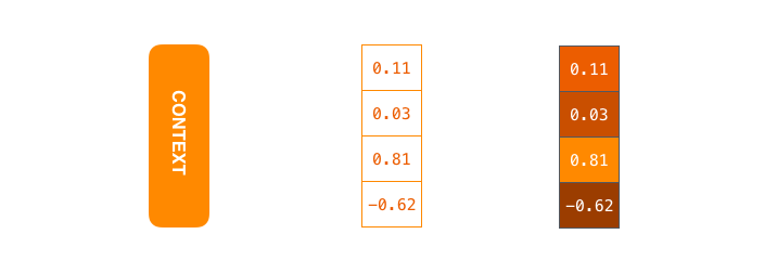
context 는 float 으로 이루어진 하나의 벡터입니다. 우리의 시각화 예시에서는 더 높은 값을 가지는 소수를 더 밝게 표시할 예정입니다. The context is a vector of floats. Later in this post we will visualize vectors in color by assigning brighter colors to the cells with higher values.
이 context 벡터의 크기는 모델을 처음 설정할 때 원하는 값으로 설정할 수 있습니다. 하지만 보통 encoder RNN의 hidden unit 개수로 정합니다. 이 글의 시각화 예시에서는 크기 4의 context 벡터를 이용하는데요, 실제 연구에서는 256, 512, 1024 와 같은 숫자를 이용합니다. You can set the size of the context vector when you set up your model. It is basically the number of hidden units in the encoder RNN. These visualizations show a vector of size 4, but in real world applications the context vector would be of a size like 256, 512, or 1024.
Seq2seq 모델 디자인을 보게 되면 하나의 RNN 은 한 타임 스텝마다 두 개의 입력을 받습니다. 하나는 sequence 의 한 아이템이고 다른 하나는 그전 스텝에서의 RNN의 hidden state입니다. 이 두 입력들은 RNN에 들어가기 전에 꼭 vector로 변환 되어야 합니다. 하나의 단어를 벡터로 바꾸기 위해서 우리는 “word embedding” 이라는 기법을 이용합니다. 이 기법을 통해 단어들은 벡터 공간에 투영되고, 그 공간에서 우리는 단어 간 다양한 의미와 관련된 정보들을 알아낼 수 있습니다. (가장 유명한 예로 다음 식이 있습니다: king - man + woman = queen).
By design, a RNN takes two inputs at each time step: an input (in the case of the encoder, one word from the input sentence), and a hidden state. The word, however, needs to be represented by a vector. To transform a word into a vector, we turn to the class of methods called “word embedding” algorithms. These turn words into vector spaces that capture a lot of the meaning/semantic information of the words (e.g. king - man + woman = queen).
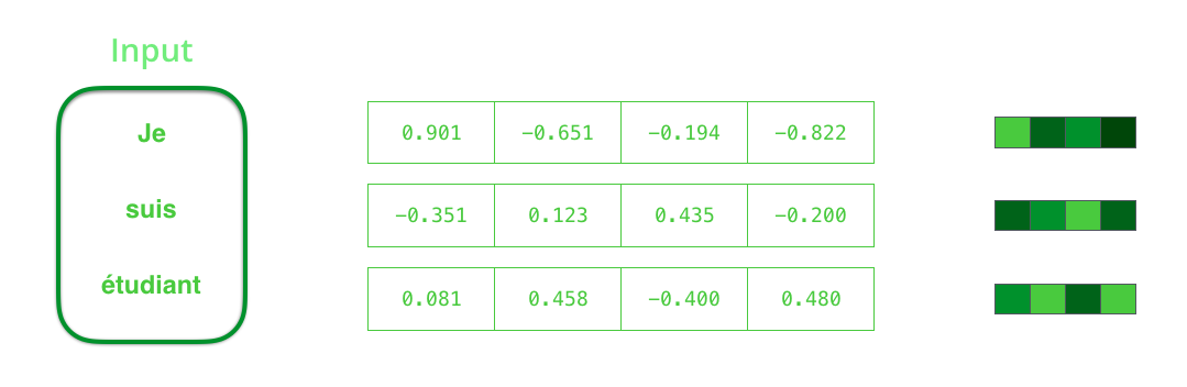
앞서 설명한 대로 encoder에서 단어들을 처리하기 전에 먼저 벡터들로 변환해주어야 합니다. 우리는 word embedding 알고리즘을 이용해 변환합니다. 또한 우리는 pre-trained embeddings 을 이용하거나 우리가 가진 데이터 셋을 이용해 직접 학습시킬 수 있습니다. 보통 크기 200 혹은 300의 embedding 벡터를 이용하지만, 이 포스트에서는 예시로서 크기 4의 벡터를 이용합니다. We need to turn the input words into vectors before processing them. That transformation is done using a word embedding algorithm. We can use pre-trained embeddings or train our own embedding on our dataset. Embedding vectors of size 200 or 300 are typical, we’re showing a vector of size four for simplicity.
여기까지 모델에서 등장하는 주요 벡터들을 소개해보았는데요, 이제 RNN의 원리에 대해서 간단히 다시 돌아보고 시각화에서 우리가 쓸 기호들을 설명하겠습니다: Now that we’ve introduced our main vectors/tensors, let’s recap the mechanics of an RNN and establish a visual language to describe these models:
이와 같이 타임 스텝 #2 에서는 두번째 단어와 첫 번째 hidden state을 이용하여 두 번째 출력을 만듭니다. 본 포스트의 뒷부분에서는, 이와 유사한 애니메이션을 이용해 신경망 기계 번역 모델을 설명하겠습니다. The next RNN step takes the second input vector and hidden state #1 to create the output of that time step. Later in the post, we’ll use an animation like this to describe the vectors inside a neural machine translation model.
밑의 영상을 보시면, encoder 혹은 decoder 에서 일어나는 각 진동은 한 번의 스텝 동안 출력을 만들어내는 과정을 의미합니다. encoder 와 decoder 는 모두 RNN이며, RNN은 한번 아이템을 처리할 때마다 새로 들어온 아이템을 이용해 그의 hidden state를 업데이트 합니다. 이 hidden state 는 그에 따라 encoder 가 보는 입력 시퀀스 내의 모든 단어에 대한 정보를 담게 됩니다. In the following visualization, each pulse for the encoder or decoder is that RNN processing its inputs and generating an output for that time step. Since the encoder and decoder are both RNNs, each time step one of the RNNs does some processing, it updates its hidden state based on its inputs and previous inputs it has seen.
그러면 시각화된 encoder의 hidden states 볼까요? 여기서 한가지 짚고 넘어갈 점은 마지막 단어의 hidden state가 바로 우리가 decoder 에게 넘겨주는 context 라는 것입니다. Let’s look at the hidden states for the encoder. Notice how the last hidden state is actually the context we pass along to the decoder.
decoder 도 그만의 hidden states 를 가지고 있으며 스텝마다 업데이트를 하게 됩니다. 우리는 아직 모델의 큰 그림을 그리고 있기 때문에 위의 영상에서는 그것을 표시하지 않았습니다. The decoder also maintains a hidden states that it passes from one time step to the next. We just didn’t visualize it in this graphic because we’re concerned with the major parts of the model for now.
그렇다면 이제 이 seq2seq 모델을 다른 방법으로 시각화해보도록 하겠습니다. 아래의 영상은 이전 것들 보다 조금 더 정적인데요, 하나의 합쳐진 RNN 이 아닌 각 스텝마다 RNN 을 표시하는 방법입니다. 이렇게 하면 각 스텝마다 입력과 출력을 정확히 볼 수 있습니다. Let’s now look at another way to visualize a sequence-to-sequence model. This animation will make it easier to understand the static graphics that describe these models. This is called an “unrolled” view where instead of showing the one decoder, we show a copy of it for each time step. This way we can look at the inputs and outputs of each time step.
이제 Attention 을 해봅시다
연구를 통해 context 벡터가 이런 seq2seq 모델의 가장 큰 걸림돌인 것으로 밝혀졌습니다. 이렇게 하나의 고정된 벡터로 전체의 맥락을 나타내는 방법은 특히 긴 문장들을 처리하기 어렵게 만들었습니다. 이에 대한 해결 방법으로 제시된 것이 바로 “Attention” 입니다 Bahdanau et al., 2014 and Luong et al., 2015. 이 두 논문이 소개한 attention 메커니즘은 seq2seq 모델이 디코딩 과정에서 현재 스텝에서 가장 관련된 입력 파트에 집중할 수 있도록 해줌으로써 기계 번역의 품질을 매우 향상 시켰습니다. The context vector turned out to be a bottleneck for these types of models. It made it challenging for the models to deal with long sentences. A solution was proposed in Bahdanau et al., 2014 and Luong et al., 2015. These papers introduced and refined a technique called “Attention”, which highly improved the quality of machine translation systems. Attention allows the model to focus on the relevant parts of the input sequence as needed.
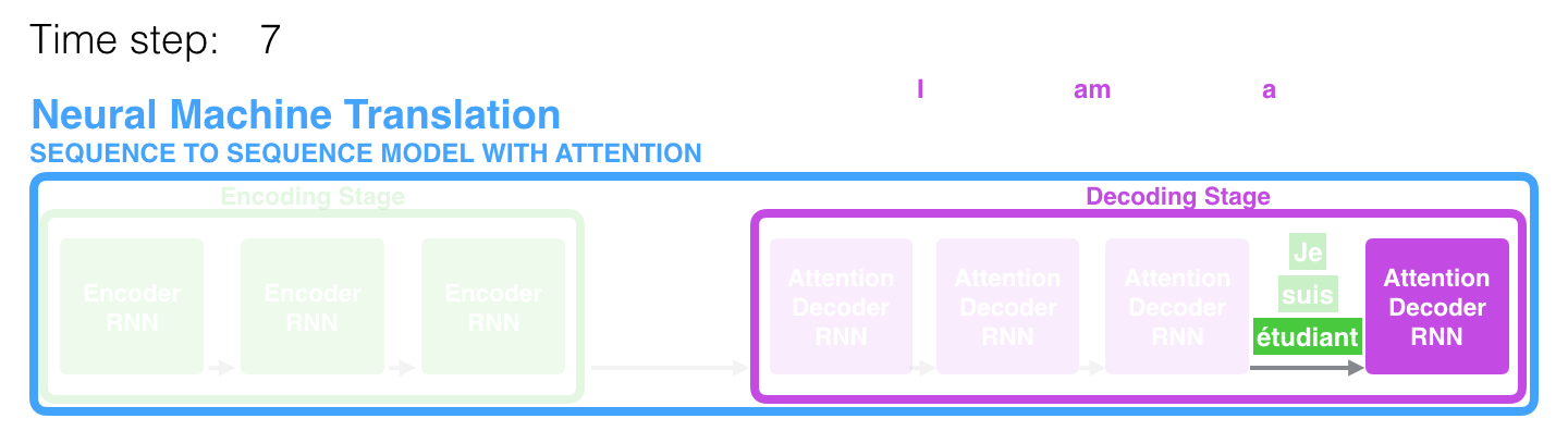
스텝 7 에서 attention 메커니즘은 영어 번역을 생성하려 할 때 decoder가 단어 “étudiant” (“학생”을 의미하는 불어)에 집중하게 합니다. 이렇게 스텝마다 관련된 부분에 더 집중할 수 있게 해주는 attention model 은 attention 이 없는 모델보다 훨씬 더 좋은 결과를 생성합니다. At time step 7, the attention mechanism enables the decoder to focus on the word “étudiant” (“student” in french) before it generates the English translation. This ability to amplify the signal from the relevant part of the input sequence makes attention models produce better results than models without attention.
계속해서 개략적인 차원에서 attention 모델을 살펴보도록 하겠습니다. attention 모델과 기존의 seq2seq 모델은 2가지의 차이점을 가집니다: Let’s continue looking at attention models at this high level of abstraction. An attention model differs from a classic sequence-to-sequence model in two main ways:
첫 번째로 encoder 가 decoder에게 넘겨주는 데이터의 양이 attention 모델에서 훨씬 더 많다는 점입니다. 기존 seq2seq 모델에서는 그저 마지막 아이템의 hidden state 벡터를 넘겼던 반면 attention 모델에서는 모든 스텝의 hidden states를 decoder에게 넘겨줍니다: First, the encoder passes a lot more data to the decoder. Instead of passing the last hidden state of the encoding stage, the encoder passes all the hidden states to the decoder:
두 번째로는 attention 모델의 decoder가 출력을 생성할 때에는 하나의 추가 과정이 필요합니다. decoder는 현재 스텝에서 관련 있는 입력을 찾아내기 위해 다음 과정을 실행합니다: Second, an attention decoder does an extra step before producing its output. In order to focus on the parts of the input that are relevant to this decoding time step, the decoder does the following:
2. 각 스텝의 hidden state마다 점수를 매깁니다 (일단 지금은 어떻게 점수를 매기는지에 대해서는 얘기하지 않겠습니다)
3. 매겨진 점수들에 softmax를 취하고 이것을 각 타임 스텝의 hidden states에 곱해서 더합니다. 이를 통해 높은 점수를 가진 hidden states는 더 큰 부분을 차지하게 되고 낮은 점수를 가진 hidden states는 작은 부분을 가져가게 됩니다.
1. Look at the set of encoder hidden states it received -- each encoder hidden states is most associated with a certain word in the input sentence
2. Give each hidden states a score (let's ignore how the scoring is done for now)
3. Multiply each hidden states by its softmaxed score, thus amplifying hidden states with high scores, and drowning out hidden states with low scores
이러한 점수를 매기는 과정은 decoder가 단어를 생성하는 매 스텝마다 반복됩니다. This scoring exercise is done at each time step on the decoder side.
이제 이때까지 나온 모든 과정들을 합친 다음 영상을 보고 어떻게 attention 이 작동하는지 정리해보겠습니다: Let us now bring the whole thing together in the following visualization and look at how the attention process works:
- attention 모델에서의 decoder RNN 은 과 추가로 initial decoder hidden state을 입력받습니다.
- decoder RNN 은 두 개의 입력을 가지고 새로운 hidden state벡터를 출력합니다. (h4). RNN의 출력 자체는 사용되지 않고 버려집니다.
- Attention 과정: encoder의 hidden state 모음과 decoder 의 hidden state h4 벡터를 이용하여 그 스텝에 해당하는 context 벡터 (C4) 를 계산합니다.
- h4 와 C4 를 하나의 벡터로 concatenate (연결, 이어쓰기) 합니다.
- 이 벡터를 feedforward 신경망 (seq2seq 모델 내에서 함께 학습되는 layer 입니다) 에 통과 시킵니다.
- feedforward 신경망에서 나오는 출력은 현재 타임 스텝의 출력 단어를 나타냅니다.
- 이 과정을 다음 타임 스텝에서도 반복합니다. The attention decoder RNN takes in the embedding of the token, and an initial decoder hidden state. The RNN processes its inputs, producing an output and a new hidden state vector (h4). The output is discarded. Attention Step: We use the encoder hidden states and the h4 vector to calculate a context vector (C4) for this time step. We concatenate h4 and C4 into one vector. We pass this vector through a feedforward neural network (one trained jointly with the model). The output of the feedforward neural networks indicates the output word of this time step. Repeat for the next time steps
이 attention 을 이용하면 각 decoding 스텝에서 입력 문장에서 어떤 부분을 집중하고 있는지에 대해 볼 수 있습니다: This is another way to look at which part of the input sentence we’re paying attention to at each decoding step:
여기서 한가지 짚고 넘어갈 것은 현재 모델이 아무 이유 없이 출력의 첫 번째 단어를 입력의 첫 번째 단어와 맞추는 (align) 것이 아니란 것입니다. 학습 과정에서 입력되는 두 개의 언어를 어떻게 맞출지는 학습이 됩니다 (우리의 예시에는 불어와 영어입니다). 얼마나 이것이 정확하게 학습 되는지를 알아보기 위해서 앞서 언급했던 attention 논문들에서는 다음과 같은 예시를 보여줍니다: Note that the model isn’t just mindless aligning the first word at the output with the first word from the input. It actually learned from the training phase how to align words in that language pair (French and English in our example). An example for how precise this mechanism can be comes from the attention papers listed above:
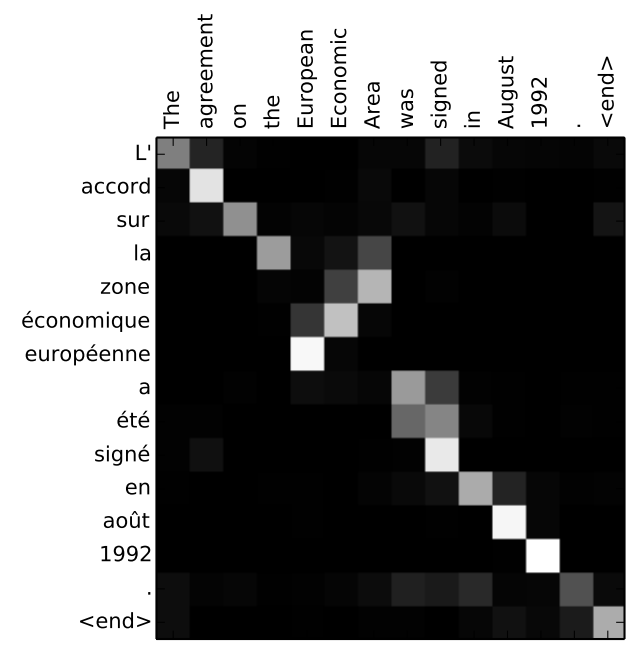
모델이 “European Economic Area”를 제대로 출력할 때 모델이 얼마나 잘 주의를 하고 있는지를 볼 수 있습니다. 영어와는 달리 불어에서는 이 단어들의 순서가 반대입니다 (“européenne économique zone”). 문장 속의 다른 단어들은 다 비슷한 순서를 가지고 있습니다. You can see how the model paid attention correctly when outputing “European Economic Area”. In French, the order of these words is reversed (“européenne économique zone”) as compared to English. Every other word in the sentence is in similar order.
이제 구현을 할 준비가 됐다고 느껴지신다면 TensorFlow의 Neural Machine Translation (seq2seq) Tutorial를 꼭 확인해보세요. If you feel you’re ready to learn the implementation, be sure to check TensorFlow’s Neural Machine Translation (seq2seq) Tutorial.
여기에 그려진 것들은 제가 Udacity에서 하고 있는 강의 Natural Language Processing Nanodegree Program의 한 수업 중 일부분입니다. 이 강의에서 관련된 응용 부분들과 Transformer 모델 (Attention Is All You Need)과 같은 attention 메커니즘을 활용한 최근 연구 등등 더욱더 자세한 것을 다루고 있으니 관심이 있으시다면 확인해보세요. I hope you’ve found this useful. These visuals are early iterations of a lesson on attention that is part of the Udacity Natural Language Processing Nanodegree Program. We go into more details in the lesson, including discussing applications and touching on more recent attention methods like the Transformer model from Attention Is All You Need.
이 글에 대해서 피드백이 있으시다면 제 트위터 아이디 @jalammmar로 연락주세요. I’d love any feedback you may have. Please reach me at @jalammmar.