The Illustrated BERT, ELMo, and co. (How NLP Cracked Transfer Learning)
저번 글에 이어 이번엔 다른 contextualized Language Model 들인 BERT와 ELMo에 대한 글을 번역해보았습니다. 마찬가지로 블로그 by Jay Alammar에서 허락을 받고 가져온 글이며, 원문은 본 링크 에서 확인하실 수 있습니다.
아래의 번역 글은 마우스를 올리시면 (모바일의 경우 터치) 원문을 확인하실 수 있습니다. 혹시 번역에 심각한 오류 혹은 오탈자를 확인하신다면 밑의 Disqus 댓글 창에 남겨주시면 감사하겠습니다.
(이하 본문)
BERT, ELMo의 시각화 (NLP에서의 Transfer Learning) by Jay Alammar
2018년은 텍스트를 다루는 머신러닝 모델들 (더 정확히는 Natural Lawngauge Processing 혹은 NLP) 에게는 아주 큰 변화가 있었던 해입니다. 어떻게 하면 가장 잘 단어와 문장을 그 아래에 있는 의미까지 나타낼 수 있을 지에 대한 우리의 이해도가 매우 빠르게 높아지고 있습니다. 뿐만 아니라, NLP 커뮤니티는 다운로드 받기만 하면 우리의 모델과 파이프라인에 쉽게 적용시킬 수 있는 매우 강력한 (부품) 모델들을 내놓고 있습니다. 이것은 NLP의 ImageNet 시기 라고 불리고 있습니다. 몇년 전 Computer Vision 테스크들에서 이와 비슷한 연구들을 통해 엄청나게 발전했기 때문이죠. The year 2018 has been an inflection point for machine learning models handling text (or more accurately, Natural Language Processing or NLP for short). Our conceptual understanding of how best to represent words and sentences in a way that best captures underlying meanings and relationships is rapidly evolving. Moreover, the NLP community has been putting forward incredibly powerful components that you can freely download and use in your own models and pipelines (It’s been referred to as NLP’s ImageNet moment, referencing how years ago similar developments accelerated the development of machine learning in Computer Vision tasks).
(ULM-FiT은 Cookie Monster와 전혀 관계가 없지만 다른 걸 생각해낼 수 없었으므로 이렇게 두도록 하겠습니다…) (ULM-FiT has nothing to do with Cookie Monster. But I couldn’t think of anything else..)
이러한 발전에 있어서 큰 마일스톤 중 가장 최근 연구는 BERT의 발표 입니다. 이 연구의 발표는 NLP의 새로운 시대를 열어갈만한 사건으로 평가 되고 있습니다. BERT 모델은 수 많은 언어와 관련된 task 에서 새로운 기록을 세웠습니다. 이 모델을 설명하는 논문과 함께, 이 연구를 진행하던 팀에서는 모델의 open-source 코드를 공개하였으며, 아주 거대한 데이터셋을 이용해 pre-train된 모델을 다운로드 가능하게 해두었습니다. 이제 누구나 이 파워풀하면서도 아주 쉽게 붙일 수 있는 component 를 이용하여 자연어 처리를 포함하는 머신 러닝 모델을 개발할 수 있게 된 것이죠 – 처음부터 학습을 시키는 것 (training from scratch)에 들어가는 엄청난 시간, 에너지, 지식, 그리고 자원을 아낄 수 있게 된 것입니다. One of the latest milestones in this development is the release of BERT, an event described as marking the beginning of a new era in NLP. BERT is a model that broke several records for how well models can handle language-based tasks. Soon after the release of the paper describing the model, the team also open-sourced the code of the model, and made available for download versions of the model that were already pre-trained on massive datasets. This is a momentous development since it enables anyone building a machine learning model involving language processing to use this powerhouse as a readily-available component – saving the time, energy, knowledge, and resources that would have gone to training a language-processing model from scratch.
BERT가 어떻게 개발되었는 지를 보여주는 두가지 스텝입니다. Step 1 에서는 pre-train된 모델을 다운로드 할 수 있으며, step 2 에서는 이제 fine-tuning에 대해서만 신경쓰면 됩니다. The two steps of how BERT is developed. You can download the model pre-trained in step 1 (trained on un-annotated data), and only worry about fine-tuning it for step 2. [Source for book icon].
BERT는 NLP 커뮤니티에 최근 떠올랐던 여러가지 영리한 아이디어를 바탕으로 하고 있습니다 – Semi-supervised Sequence Learning (by Andrew Dai and Quoc Le), ELMo (by Matthew Peters 와 AI2 연구자들과 UW CSE의 연구자들), ULMFiT (by fast.ai 창립자 Jeremy Howard와 Sebastian Ruder), OpenAI transformer (by OpenAI 연구자들 Radford, Narasimhan, Salimans, and Sutskever), Transformer (Vaswani et al). BERT builds on top of a number of clever ideas that have been bubbling up in the NLP community recently – including but not limited to Semi-supervised Sequence Learning (by Andrew Dai and Quoc Le), ELMo (by Matthew Peters and researchers from AI2 and UW CSE), ULMFiT (by fast.ai founder Jeremy Howard and Sebastian Ruder), the OpenAI transformer (by OpenAI researchers Radford, Narasimhan, Salimans, and Sutskever), and the Transformer (Vaswani et al).
BERT가 정확히 무엇인지 알기 위해서는 몇가지 개념들에 대해서 알고 있어야 합니다. 그러므로 BERT 모델 자체와 연관된 개념들을 알아보기 전에, 일단 먼저 BERT를 어떻게 이용할 수 있는지에 대해서 보도록 하겠습니다. There are a number of concepts one needs to be aware of to properly wrap one’s head around what BERT is. So let’s start by looking at ways you can use BERT before looking at the concepts involved in the model itself.
예제: 문장 분류 (Sentence Classification)
Example: Sentence Classification
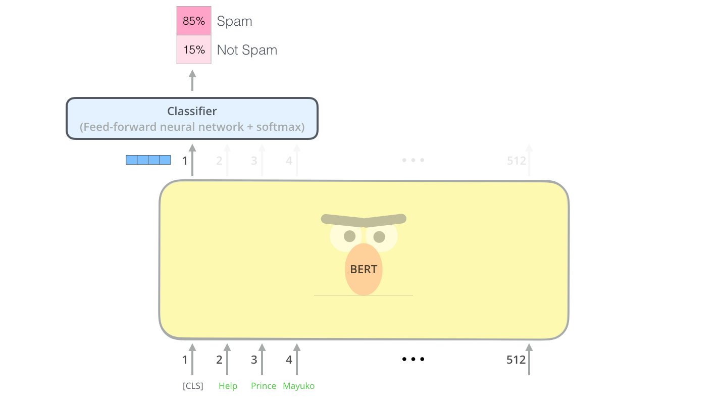
BERT를 이용하는 가장 직관적으로 간단한 방법은 하나의 text를 분류하는 것입니다. 이러한 모델은 다음과 같을 것입니다: The most straight-forward way to use BERT is to use it to classify a single piece of text. This model would look like this:
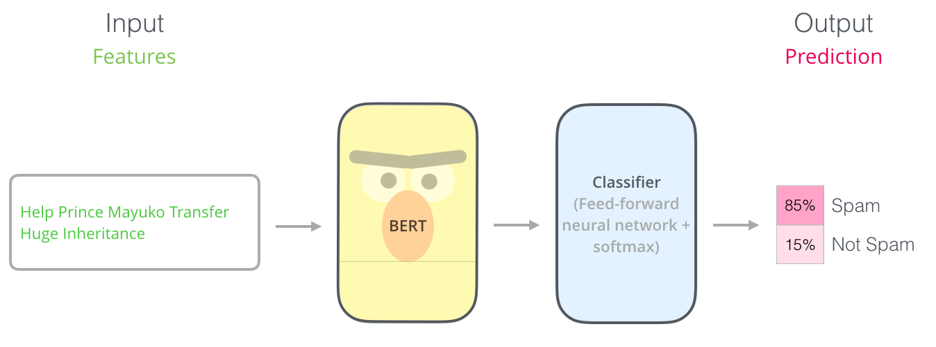
이런 모델을 학습 시키기 위해서 우리는 classifier를 train 시켜야 하는데요, 이것은 BERT 모델의 학습 과정을 최소한으로 변경하면서도 가능합니다. 이러한 학습 과정을 우리는 Fine-Tuning 이라고 부르며, Semi-supervised Sequence Learning 와 ULMFiT에 그 기원을 두고 있습니다. To train such a model, you mainly have to train the classifier, with minimal changes happening to the BERT model during the training phase. This training process is called Fine-Tuning, and has roots in Semi-supervised Sequence Learning and ULMFiT.
우리는 지금 classifier에 대해서 얘기하고 있으므로, 우리는 머신 러닝에서 supervised-learning 영억을 다루고 있는 것입니다. 즉, 우리는 이러한 모델을 학습 시키기 위해서 label이 있는 데이터 셋이 필요합니다. 예를 들어 이 스팸 분류 모델의 예제에서는 label 된 데이터 셋이란 이메일들과 각 이메일에 대한 label(“스팸”인지 “스팸이 아님”인지를 나타내는 라벨)을 나타냅니다. For people not versed in the topic, since we’re talking about classifiers, then we are in the supervised-learning domain of machine learning. Which would mean we need a labeled dataset to train such a model. For this spam classifier example, the labeled dataset would be a list of email messages and a labele (“spam” or “not spam” for each message).
이와 같은 사용 예제로는 다음이 있습니다: Other examples for such a use-case include:
- Sentiment analysis (감성 분석)
- 입력: 영화/제품 리뷰. 출력: 긍정/부정
- 예시 데이터 셋: SST
- Fact-checking (사실 확인)
- 입력: 문장. 출력: “주장함” or “주장이 아님”
- 언젠가 미래에 기대하는 출력:
- 입력: 주장이 담긴 문장 출력: “사실” or “사실이 아님”
- Full Fact은 대중들을 위해 자동 fact-checking 툴을 만드는 조직입니다. 그들의 시스템 중 한 부분은 뉴스를 읽고 그 안에 있는 주장들을 탐지하는 classifier 입니다 (텍스트를 “주장” 혹은 “주장이 아님”으로 분류합니다). 이 주장들은 모여 나중에 사실인지 아닌지 fact-check 될 수 있습니다 (현재는 사람에 의해 되고 있지만 언젠가 머신러닝으로 가능하길 기대하고 있습니다).
- 관련 비디오: 자동 fact-checking 을 위한 문장 embedding - Lev Konstantinovskiy. Sentiment analysis Input: Movie/Product review. Output: is the review positive or negative? Example dataset: SST Fact-checking Input: sentence. Output: “Claim” or “Not Claim” More ambitious/futuristic example: Input: Claim sentence. Output: “True” or “False” Full Fact is an organization building automatic fact-checking tools for the benefit of the public. Part of their pipeline is a classifier that reads news articles and detects claims (classifies text as either “claim” or “not claim”) which can later be fact-checked (by humans now, by with ML later, hopefully). Video: Sentence embeddings for automated factchecking - Lev Konstantinovskiy.
모델 구조
이제 어떻게 BERT를 쓸 수 있을지 사용 예제가 머리에 있을테니, 이제 이 모델이 어떻게 작동하는지를 조금 더 제대로 알아보도록 하겠습니다. Now that you have an example use-case in your head for how BERT can be used, let’s take a closer look at how it works.
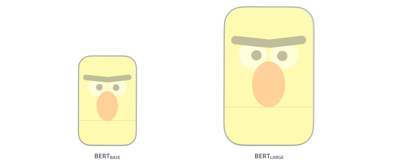
BERT 논문은 두 개의 사이즈의 모델을 소개합니다: The paper presents two model sizes for BERT:
- BERT BASE – 이전의 OpenAI Transformer와 성능을 비교하기 위해 설정된 사이즈
- BERT LARGE – 논문에 명시된 state-of-the-art 결과들을 얻게 해 준 말도 안되게 큰 사이즈의 모델 BERT BASE – Comparable in size to the OpenAI Transformer in order to compare performance BERT LARGE – A ridiculously huge model which achieved the state of the art results reported in the paper
BERT는 단순히 말하자면 학습된 Transformer Encoder를 쌓아 놓은 것입니다. 앞으로 설명할 BERT의 기본 개념인 Transformer model 에 대해서 익숙하지 않으시다면 이전 글인 The Illustrated Transformer를 꼭 참고하세요. BERT is basically a trained Transformer Encoder stack. This is a good time to direct you to read my earlier post The Illustrated Transformer which explains the Transformer model – a foundational concept for BERT and the concepts we’ll discuss next.
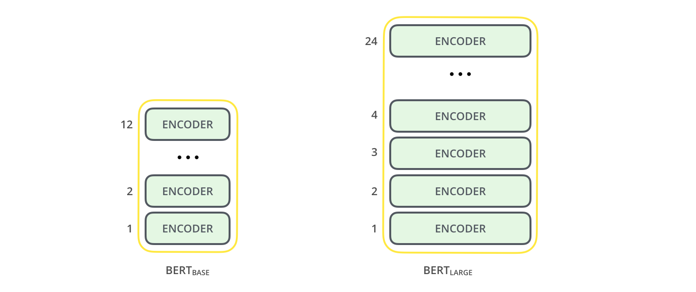
BERT의 두 모델 크기 모두 매우 많은 수의 encoder layer를 가지고 있습니다 (논문에서는 Transformer Blocks라고 부릅니다) – Base 버전에는 12개를 가지며 Large version 에서는 24개를 가집니다. feedforward-network의 크기 또한 매우 크고 (768과 1024개의 hidden unit) Transformer의 첫 논문에 나온 구현 설정 (6개의 encoder layers, 512개의 hidden units, 8개의 attention heads) 보다도 많은 attention heads를 가지고 있습니다. Both BERT model sizes have a large number of encoder layers (which the paper calls Transformer Blocks) – twelve for the Base version, and twenty four for the Large version. These also have larger feedforward-networks (768 and 1024 hidden units respectively), and more attention heads (12 and 16 respectively) than the default configuration in the reference implementation of the Transformer in the initial paper (6 encoder layers, 512 hidden units, and 8 attention heads).
Model Inputs
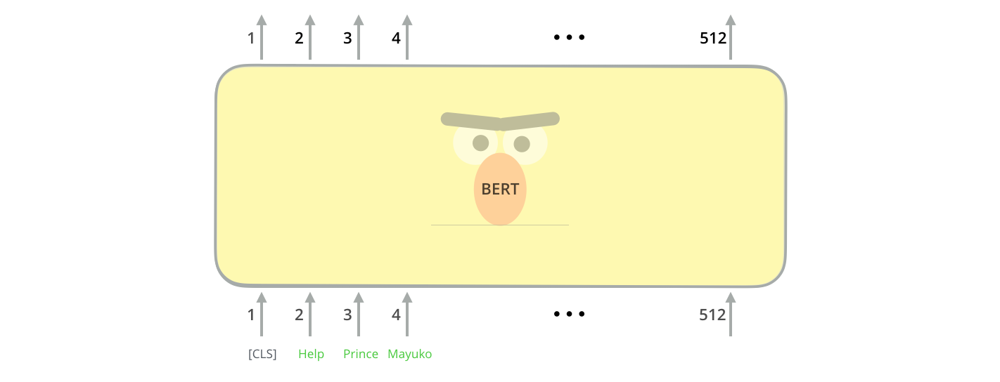
첫 번째 입력 토큰으로는 스페셜 토큰인 [CLS]가 들어가게 됩니다. 이렇게 하는 이유는 나중에 자연스럽게 알게될 것입니다. 여기서 CLS란 Classification을 나타냅니다. The first input token is supplied with a special [CLS] token for reasons that will become apparent later on. CLS here stands for Classification.
transformer의 기본 encoder와 동일하게, BERT는 단어의 시퀀스를 입력으로 받아 encoder stack을 계속 타고 올라갑니다. 각 encoder layer는 self-attention을 적용하고 feed-forward network를 통과시킨 결과를 다음 encoder에게 전달합니다. Just like the vanilla encoder of the transformer, BERT takes a sequence of words as input which keep flowing up the stack. Each layer applies self-attention, and passes its results through a feed-forward network, and then hands it off to the next encoder.
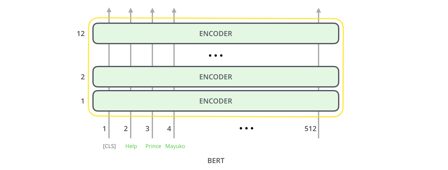
구조상 보았을 때, 현재 encoding 단계까지는 Transformer와 동일합니다 (언제든 조절할 수 있는 모델 안의 hidden unit수와 같은 size 제외). 이제 출력 단계로 넘어가면 어떻게 BERT와 Transformer가 다른지를 볼 수 있게 됩니다. In terms of architecture, this has been identical to the Transformer up until this point (aside from size, which are just configurations we can set). It is at the output that we first start seeing how things diverge.
Model Outputs
각 (단어) 위치에서는 hidden_size의 (BERT Base의 경우 768) 벡터를 출력합니다. 위에서 살펴본 문장 분류 (sentence classification) 예제의 경우, 우리는 첫 번째 위치에서의 출력 (output)에만 집중합니다. 이것은 바로 스페셜 토큰인 [CLS]의 결과이죠. Each position outputs a vector of size hidden_size (768 in BERT Base). For the sentence classification example we’ve looked at above, we focus on the output of only the first position (that we passed the special [CLS] token to).
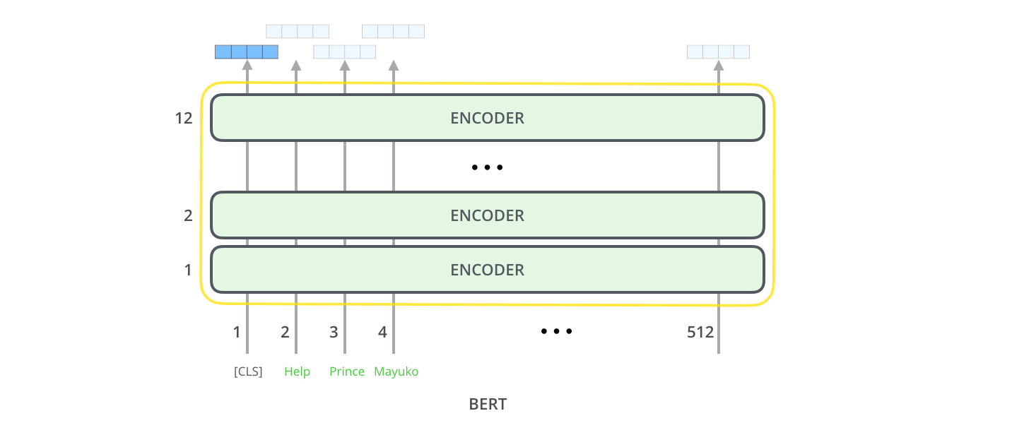
결과로 나온 출력 벡터는 이제 우리가 고른 classifier에 입력으로 이용될 수 있습니다. BERT의 논문에서는 매우 단순한 형태인 single-layer를 classifier로 이용했음에도 불구하고 매우 좋은 결과를 얻었습니다. That vector can now be used as the input for a classifier of our choosing. The paper achieves great results by just using a single-layer neural network as the classifier.
만약 이용하고 싶은 task가 더 다양한 종류의 label을 가진다면 (예를 들어, email을 “spam”,”not spam”, “social”, “promotion” 네가지 label으로 분류하고 싶은 경우), 그저 classifier network를 조금 변형해주어 더 많은 output neurons를 가지게 하고 softmax를 통과시키면 됩니다. If you have more labels (for example if you’re an email service that tags emails with “spam”, “not spam”, “social”, and “promotion”), you just tweak the classifier network to have more output neurons that then pass through softmax.
Convolutional Networks와의 유사점
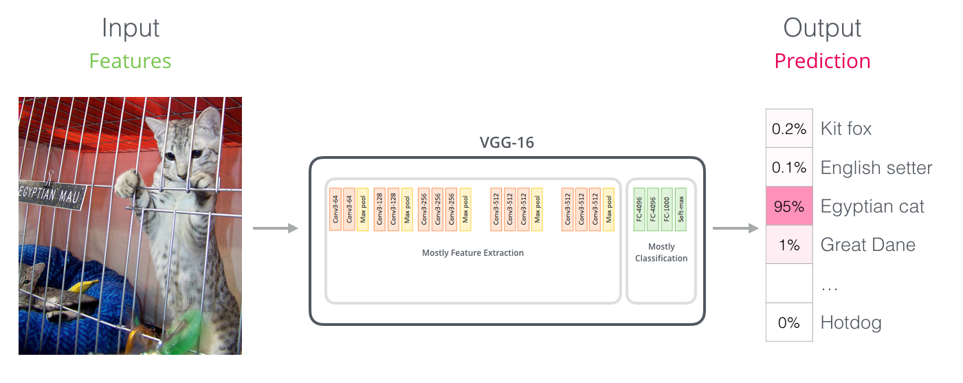
만약 computer vision을 조금 아시는 분이라면, BERT에서 이 마지막 벡터를 활용하는 모습이 VGGNet과 같은 convolution 부분의 결과를 마지막 fully-connected classification 부분에서 이용하는 모습과 유사한다는 것을 느끼실 수 있을 것입니다. For those with a background in computer vision, this vector hand-off should be reminiscent of what happens between the convolution part of a network like VGGNet and the fully-connected classification portion at the end of the network.
드디어 새로운 Embedding의 시대가 왔습니다.
ELMo와 BERT와 같은 새로운 연구들은 이제 단어가 어떻게 encode 될 수 있는지 자체를 바꾸게 될 것입니다. 이전까지, word-embedding은 언어를 처리하는 NLP 모델들의 아주 큰 힘이 되어 왔습니다. Word2Vec과 Glove와 같은 방법들은 많은 task들에서 광범위하게 사용되어 왔습니다. 먼저 이 word-embedding들이 어떻게 이용되어 왔는지를 잠시 복습하고 이제 이것이 어떻게 변하게 될 지 알아보도록 하겠습니다. These new developments carry with them a new shift in how words are encoded. Up until now, word-embeddings have been a major force in how leading NLP models deal with language. Methods like Word2Vec and Glove have been widely used for such tasks. Let’s recap how those are used before pointing to what has now changed.
Word Embedding 복습
머신 러닝 모델들이 단어를 처리하고 계산에 이용하기 위해서는, 이 단어들을 숫자로 표현 (numeric representation)을 해야만 합니다. Word2vec는 벡터 (숫자들의 리스트) 를 이용하면 제대로 단어의 의미와 의미와 관련된 관계 (e.g., 단어들이 비슷한지 혹은 반대인지, 혹은 “Stockholm”과 “Sweden”이 “Cairo”과 “Egypt”와 동일한 관계를 가지는지) 그리고 문법과 문법과 관련된 관계 (e.g., “had”와 “has”가 가지는 관계와 “was”와 “is”가 가지는 관계가 같은지) 를 나타낼 수 있음을 보였습니다. For words to be processed by machine learning models, they need some form of numeric representation that models can use in their calculation. Word2Vec showed that we can use a vector (a list of numbers) to properly represent words in a way that captures semantic or meaning-related relationships (e.g. the ability to tell if words are similar, or opposites, or that a pair of words like “Stockholm” and “Sweden” have the same relationship between them as “Cairo” and “Egypt” have between them) as well as syntactic, or grammar-based, relationships (e.g. the relationship between “had” and “has” is the same as that between “was” and “is”).
사람들은 매우 빠르게 모델이 이용하는 작은 데이터셋에서 처음부터 학습시키는 것보다도 아주 많은 양의 텍스트 데이터에서 pre-train된 embedding 을 이용하는게 좋다는 것을 알아내었습니다. 그래서 이제 이러한 Word2Vec 혹은 GloVe와 같은 알고리즘들을 이용해 pre-train된 단어들의 embedding을 다운받는게 가능해졌습니다. 아래는 “stick”이라는 단어의 GloVe embedding 예제입니다 (여기서 사용한 벡터의 사이즈는 200입니다) The field quickly realized it’s a great idea to use embeddings that were pre-trained on vast amounts of text data instead of training them alongside the model on what was frequently a small dataset. So it became possible to download a list of words and their embeddings generated by pre-training with Word2Vec or GloVe. This is an example of the GloVe embedding of the word “stick” (with an embedding vector size of 200)

단어 “stick”의 GloVe word embedding - 200개의 float (둘째 자리에서 반올림) 으로 이루어져있습니다. The GloVe word embedding of the word “stick” - a vector of 200 floats (rounded to two decimals). It goes on for two hundred values.
200개의 숫자는 너무 많으므로, 여기서는 다음과 같은 간단한 형태의 그림을 이용해서 word embedding 벡터를 나타내도록 하겠습니다: Since these are large and full of numbers, I use the following basic shape in the figures in my posts to show vectors:

ELMo: 우리 이제 Context 를 고려해야 함!
만약 우리가 GloVe representation을 이용한다면, 이 “stick”이라는 단어는 그 어떤 맥락 (context)에서도 같은 벡터로 나타내질 것입니다. “엥 잠시만 “stick” 은 어떻게 이용 되냐에 따라 여러 의미를 가지잖아?”라고 여러 NLP 연구자 들이 말했습니다 (Peters et. al., 2017, McCann et. al., 2017, Peters et. al., 2018 in the ELMo paper ). “그러지 말고 어떤 맥락에 있는지에 따라 다른 embedding을 이용하는게 어떨까? – 맥락 속의 단어의 의미 뿐만 아니라 맥락 자체에 대한 정보도 나타낼 수 있는 embedding!”. 그렇게 contextualized word-ebmedding이 탄생했습니다. If we’re using this GloVe representation, then the word “stick” would be represented by this vector no-matter what the context was. “Wait a minute” said a number of NLP researchers (Peters et. al., 2017, McCann et. al., 2017, and yet again Peters et. al., 2018 in the ELMo paper ), “stick”” has multiple meanings depending on where it’s used. Why not give it an embedding based on the context it’s used in – to both capture the word meaning in that context as well as other contextual information?”. And so, contextualized word-embeddings were born.
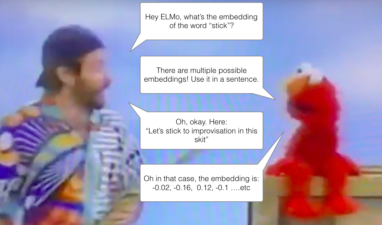
contextualized word-embeddings은 각 단어에게 문장의 맥락 속에서 어떠한 의미를 가지는지에 따라 다른 embedding을 가지게 할 수 있습니다. Contextualized word-embeddings can give words different embeddings based on the meaning they carry in the context of the sentence. Also, RIP Robin Williams
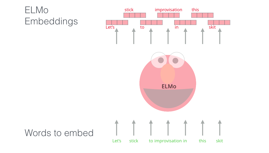
각 단어에 고정된 embedding을 이용하는 대신에, ELMo는 먼저 전체 문장을 봅니다. 그리고 특정한 task으로 학습된 bi-directional LSTM을 이용하여 각 단어의 embedding을 생성합니다. Instead of using a fixed embedding for each word, ELMo looks at the entire sentence before assigning each word in it an embedding. It uses a bi-directional LSTM trained on a specific task to be able to create those embeddings.
ELMo는 NLP의 pre-training에 있어서 중요한 한 걸음을 한 셈입니다. ELMo가 이용하는 LSTM은 거대한 데이터 셋에서 학습되며, 그 다음 자연어를 처리하는 다른 모델에서 하나의 부분으로 이용할 수 있습니다. ELMo provided a significant step towards pre-training in the context of NLP. The ELMo LSTM would be trained on a massive dataset in the language of our dataset, and then we can use it as a component in other models that need to handle language.
그렇다면 ELMo의 비밀은 무엇일까요? What’s ELMo’s secret?
ELMo는 단어의 sequence에서 다음 단어를 예측하는 task 인 Language Modeling 에서 언어에 대한 이해를 습득합니다. 이 Task가 특히 좋은 이유는 다음 단어를 label로 쓰기 때문에 사람의 도움 (human annotation) 없이 세상에 있는 엄청난 양의 모든 텍스트 데이터를 학습 데이터로 이용할 수 있다는 점입니다. ELMo gained its language understanding from being trained to predict the next word in a sequence of words - a task called Language Modeling. This is convenient because we have vast amounts of text data that such a model can learn from without needing labels.
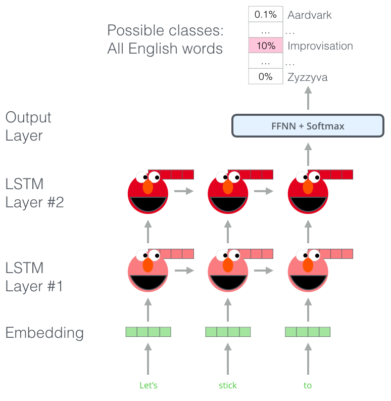
ELMo의 training 전단계: 입력으로 “계속 지켜”가 주어졌을 때, 그 다음으로 올 확률이 가장 높은 단어를 예측하기 – 이것이 바로 language modeling task 입니다. 큰 데이터 셋에 학습되었을 때, 모델은 문장들에서 언어의 패턴을 학습하기 시작합니다. 사실 방금 주어진 예제에서는 정확하게 다음 단어를 예측할 가능성이 낮습니다. 더 쉬운 예제로는, “나가서”라는 단어 다음에, “카메라”와 같은 단어 보다는 “놀자”와 같은 단어에 더 높은 확률을 주는 것이죠. A step in the pre-training process of ELMo: Given “Let’s stick to” as input, predict the next most likely word – a language modeling task. When trained on a large dataset, the model starts to pick up on language patterns. It’s unlikely it’ll accurately guess the next word in this example. More realistically, after a word such as “hang”, it will assign a higher probability to a word like “out” (to spell “hang out”) than to “camera”.
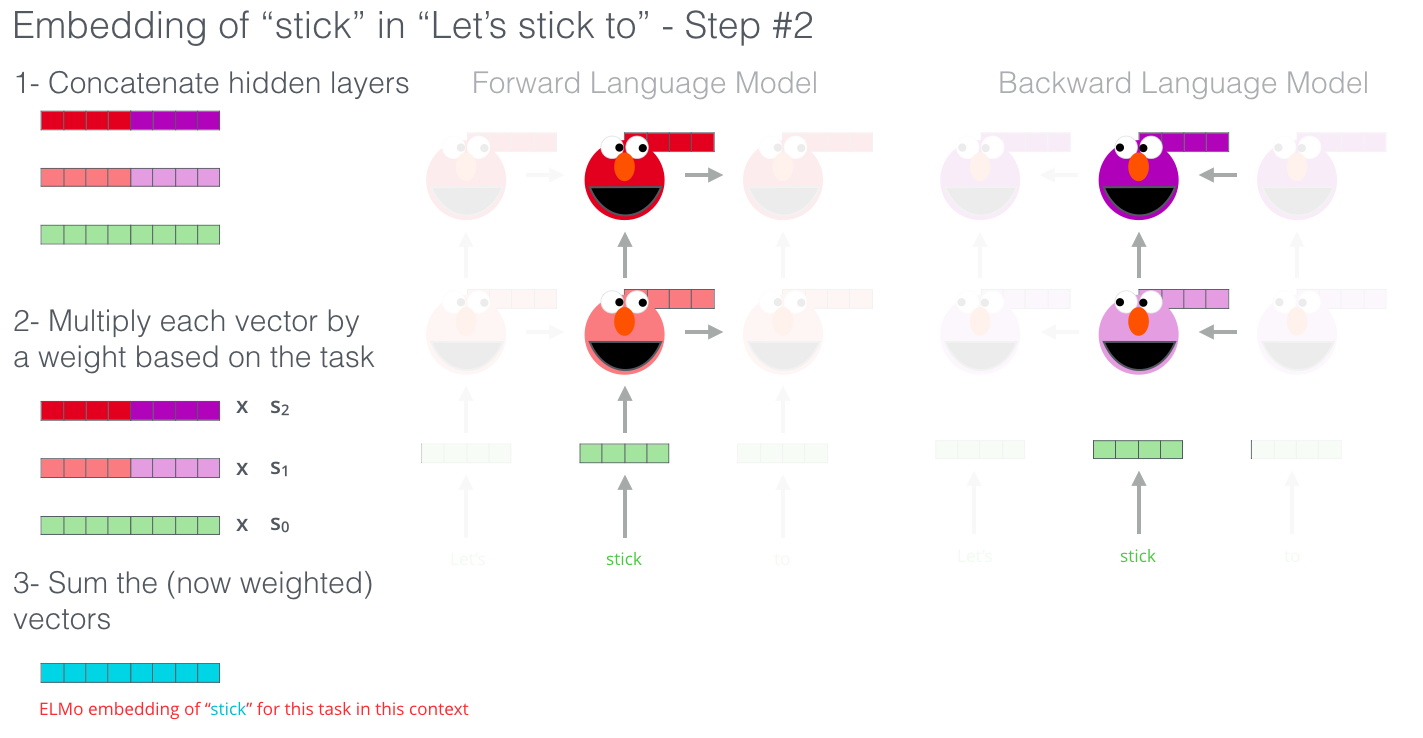
LSTM의 각 스텝을 보면, ELMo 뒤에 있는 hidden state 이 보이죠. 이것들이 바로 pre-training 이 끝난 후 임베딩을 할 때 실제로 매우 유용하게 쓰입니다. We can see the hidden state of each unrolled-LSTM step peaking out from behind ELMo’s head. Those come in handy in the embedding proecss after this pre-training is done.
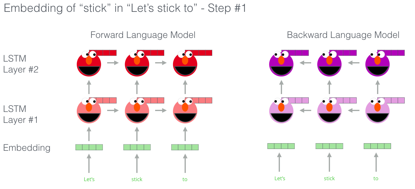
이 뿐만이 아니라 ELMo 모델은 다른 큰 장점이 있습니다. 바로 bi-directional LSTM 을 사용하는 것이죠. uni-direction 이 아닌 bi-direction 을 모두 봄으로써 이제 language model 은 단순히 다음 단어에 대해서만 추측을 하는 것이 아니라, 그 전 단어에 대해서도 이해할 수 있게 됩니다. ELMo actually goes a step further and trains a bi-directional LSTM – so that its language model doesn’t only have a sense of the next word, but also the previous word.
마지막으로, ELMo는 앞에서 보았던 hidden state들을 하나의 벡터로 합쳐서 contextualized embedding 이라고 부릅니다. 합치는 방법으로, 논문에서는 hidden state들을 concatenate (붙여쓰기)를 한 후 weighted sum 을 구하는 방식을 제안했습니다. ELMo comes up with the contextualized embedding through grouping together the hidden states (and initial embedding) in a certain way (concatenation followed by weighted summation).
ULM-FiT: NLP에서 Transfer learning 제대로 하기
ULM-FiT은 pre-training 과정에서 모델이 배우는 많은 것들을 효과적으로 활용하는 방법을 제안했습니다. 단순히 pre-training 에서 나온 embedding 혹은 contextualized embedding 을 쓰는 것이 아니라, 그 모델 자체를 활용하는 방법을 고안한 것입니다. 더 자세히 말하자면, ULM-FiT은 다양한 task들에 대해 학습된 language model을 효과적으로 fine-tune (target task에 맞도록 마지막 세부 튜닝을 해주는 것) 하는 과정을 소개하였습니다. ULM-FiT introduced methods to effectively utilize a lot of what the model learns during pre-training – more than just embeddings, and more than contextualized embeddings. ULM-FiT introduced a language model and a process to effectively fine-tune that language model for various tasks.
NLP가 드디어 Computer Vision 처럼 transfer learning 을 하는 방법을 찾은 것이죠! NLP finally had a way to do transfer learning probably as well as Computer Vision could.
Transformer: LSTM을 뛰어 넘어서
트랜스포머 모델의 논문과 코드가 공개된 후에, 사람들은 기계번역 등과 같은 여러 테스크들에서 매우 좋은 결과를 얻은 것을 보고, 이제 트랜스포머가 LSTM을 대체할 것이라고 생각하였습니다. 이것은 트랜스포머가 LSTM 보다 long-term dependencies (장기적인 정보)를 더 잘 저장하는 사실 때문이기도 했죠. The release of the Transformer paper and code, and the results it achieved on tasks such as machine translation started to make some in the field think of them as a replacement to LSTMs. This was compounded by the fact that Transformers deal with long-term dependancies better than LSTMs.
트랜스포머의 encoder-decoder 구조는 기계변역에 최적이었습니다. 하지만, 이 똑같은 구조를 문장 분류에 이용할 수 있을까요? 어떻게 이 트랜스포머 구조를 language model 으로 만들어서 pre-train 시키고 나중에 다른 테스크들에 fine-tune 시킬 수 있을까요? (나중에 실제로 supervised-learning 으로 최종적으로 잘 perform 하고자 하는 테스크들을 downstream 테스크라고 부릅니다) The Encoder-Decoder structure of the transformer made it perfect for machine translation. But how would you use it for sentence classification? How would you use it to pre-train a language model that can be fine-tuned for other tasks (downstream tasks is what the field calls those supervised-learning tasks that utilize a pre-trained model or component).
OpenAI Transformer: Language Modeling 을 위한 트랜스포머 디코더를 pre-train 시키는 방법
우리가 원하는 것은 NLP에서 transfer learning을 가능하게 하기 위한 fine-tune 할 수 있는 language model 입니다. 사람들의 고민 결과, 우리는 트랜스포머의 encoder-decoder 구조의 전체가 필요하지 않다는 결론을 내립니다. decoder 부분만으로도 할 수 있습니다. 다시 transformer에 대해서 생각해보면
It turns out we don’t need an entire Transformer to adopt transfer learning and a fine-tunable language model for NLP tasks. We can do with just the decoder of the transformer. The decoder is a good choice because it’s a natural choice for language modeling (predicting the next word) since it’s built to mask future tokens – a valuable feature when it’s generating a translation word by word.
OpenAI 트랜스포머는 decoder를 쌓아서 만듭니다. The OpenAI Transformer is made up of the decoder stack from the Transformer
더 자세히 살펴보면, 모델 안에는 총 열두개의 decoder 층이 쌓여있습니다. 여기엔 encoder가 없으므로, 기존 트랜스포머 모델에 있었던 encoder와 decoder를 이어주는 attention 층이 없음을 볼 수 있습니다. 하지만, decoder 내에는 여전히 self-attention 층이 있습니다 (당연히 decoder 내이므로 다음 단어들을 볼 수 없도록 mask 처리가 되어있습니다). The model stacked twelve decoder layers. Since there is no encoder in this set up, these decoder layers would not have the encoder-decoder attention sublayer that vanilla transformer decoder layers have. It would still have the self-attention layer, however (masked so it doesn’t peak at future tokens).
이제 language modeling 테스크로 이러한 구조를 가진 모델을 학습시킬 차례입니다. 쉽게 구할 수 있는 아주 많은 (그리고 레이블이 달려있지 않은) 텍스트를 이용해서 다음 단어를 예측하는 테스크죠. 간단합니다, 모델에 그냥 7천개의 책에 해당하는 텍스트를 던져넣고 학습하게 하면 됩니다! 책의 텍스트는 이런 종류의 테스크에 매우 적합한데요, 왜냐하면 문장들이 평균적으로 긴 편이며 한 권의 책이 모두 하나의 관련된 이야기로 채워져 있기 때문입니다. 그래서 모델들이 전반적으로 관련된 정보들을 배울 수 있게 됩니다. 트윗이나 짧은 아티클로 학습 시키는 경우에는 얻을 수 없는 좋은 점이죠. With this structure, we can proceed to train the model on the same language modeling task: predict the next word using massive (unlabeled) datasets. Just, throw the text of 7,000 books at it and have it learn! Books are great for this sort of task since it allows the model to learn to associate related information even if they’re separated by a lot of text – something you don’t get for example, when you’re training with tweets, or articles.
OpenAI 트랜스포머는 이제 7천개의 책으로 이루어진 데이터로 학습시킬 준비가 되었습니다. The OpenAI Transformer is now ready to be trained to predict the next word on a dataset made up of 7,000 books.
Downstream 테스크들에 Transfer Learning 적용하기
이제 OpenAI 트랜스포머의 모델이 pre-trained 되었습니다. 모델의 각 층 (layer)은 언어를 어느정도 잘 처리할 수 있도록 학습이 되었습니다. 이제 이 모델을 downstream 테스크들에 적용할 수 있습니다. 먼저 문장 분류 (sentence classification) 테스크의 예제를 살펴보도록 하겠습니다 (문장 분류의 예시로, 이메일이 주어졌을 때 그것이 “스팸” 인지 “스팸아님” 인지를 분류하는 것이 있습니다): Now that the OpenAI transformer is pre-trained and its layers have been tuned to reasonably handle language, we can start using it for downstream tasks. Let’s first look at sentence classification (classify an email message as “spam” or “not spam”):
문장 분류 task를 위해 pre-train된 OpenAI 트랜스포머 사용하는 법 How to use a pre-trained OpenAI transformer to do sentence clasification
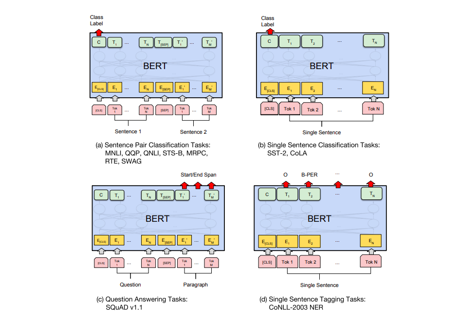
OpenAI 모델의 논문에서는 다양한 종류의 테스크들에 있어서 입력을 처리하는 방법으로 여러가지 변형 방법을 (transformation) 보여주었습니다. 논문에서 발췌한 아래의 그림은 각각의 서로 다른 테스크들에 어떻게 입력 데이터를 변형해주고 모델을 적용하는지를 보여주고 있습니다. The OpenAI paper outlines a number of input transformations to handle the inputs for different types of tasks. The following image from the paper shows the structures of the models and input transformations to carry out different tasks.
정말 기발하지 않나요? Isn’t that clever?
BERT: Decoder 에서 Encoder 으로
OpenAI 트랜스포머 모델은 우리에게 나중에 fine-tune 할 수 있는 pre-train된 모델을 제시했습니다. 하지만, LSTM에서 Transformer로 완전히 넘어가기엔 아직 문제가 있습니다. ELMo의 language model을 bi-directional (양쪽의 단어를 모두 봄) 했는데, openAI의 트랜스포머는 오직 한 방향, 즉 forward language model만 학습시킨다는 점입니다. 트랜스포머를 베이스로 하면서도 양쪽 방향을 모두 보는 모델을 만들 순 없는 걸까요 (이걸 테크니컬한 용어로 “오른쪽과 왼쪽, 즉 양쪽 방향의 맥락에 condition 되었다”고 합니다)? The openAI transformer gave us a fine-tunable pre-trained model based on the Transformer. But something went missing in this transition from LSTMs to Transformers. ELMo’s language model was bi-directional, but the openAI transformer only trains a forward language model. Could we build a transformer-based model whose language model looks both forward and backwards (in the technical jargon – “is conditioned on both left and right context”)?
“내 맥주 들어줘”, 성인 버전의 BERT가 말했습니다. “Hold my beer”, said R-rated BERT.
Masked Language Model 이란?
“우리는 transformer를 encoder로 쓸거야”, BERT가 말했습니다. “We’ll use transformer encoders”, said BERT.
Ernie 는 답장했습니다. “이건 말도 안돼. 우리 모두가 알고 있듯이, bidirectional 하게 한 단어를 본다면, 각 단어는 결국 간접적으로 여러층에서 나타나는 맥락에서 자기 자신을 보게될거야.” “This is madness”, replied Ernie, “Everybody knows bidirectional conditioning would allow each word to indirectly see itself in a multi-layered context.”
“괜찮아. 우린 mask를 쓸거니까”, BERT가 비밀스럽게 말했습니다. “We’ll use masks”, said BERT confidently.
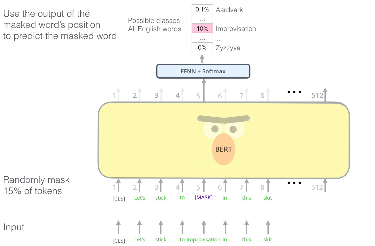
BERT는 기발하면서도 새로운 language modeling 테스크를 제안합니다. 바로 입력 텍스트에서 15%의 단어를 가려버리고 (masking), 모델에게 그 가려진 단어들을 알아맞추라고 하는 것이죠. BERT’s clever language modeling task masks 15% of words in the input and asks the model to predict the missing word.
사실 Transformer의 Encoder 부분을 language model에 활용할 수 없었던 가장 큰 이유는 기존 language modeling 테스크 자체가 트랜스포머의 encoder에 적합하지 않았기 때문입니다. language modeling 은 알 수 없는 다음의 단어를 예측하는 테스크라면, 트랜스포머의 encoder는 self-attention 층에서 모든 단어들을 봐야했기 때문이죠. BERT는 기존 task를 살짝 변형한 (이전에는 Cloze task라고 불리던) “masked language model”라는 개념을 빌려와서 문제를 해결합니다. Finding the right task to train a Transformer stack of encoders is a complex hurdle that BERT resolves by adopting a “masked language model” concept from earlier literature (where it’s called a Cloze task).
단순히 입력의 15%를 마스킹하는 것 뿐만아니라, BERT는 나중에 fine-tune 하는 과정을 위해서 몇가지 다른 task들을 추가했는데요. 예를 들어, 마스킹할 때 그저 단어를 없애는 것이 아니라 랜덤하게 뽑은 다른 단어로 바꿔치기 하여서 모델에게 원래의 맞는 단어를 예측하게 하기도 합니다. Beyond masking 15% of the input, BERT also mixes things a bit in order to improve how the model later fine-tunes. Sometimes it randomly replaces a word with another word and asks the model to predict the correct word in that position.
두개의 문장을 이용한 테스크들
OpenAI의 트랜스포머의 경우를 다시 생각해보면, 단어간의 관계를 묻는 languuage modeling 테스크 말고는 다른 테스크를 고려하지 않았죠. 하지만 downstream 테스크들 중에서는 문장들간의 관계를 묻는 테스크들도 꽤 있습니다. 예를 들어, 두 문장을 주고 그들이 서로 같은 의미를 가지는지를 묻는 phrase detection 혹은 위키피디아의 지문 하나와 질문 하나를 주고 주어진 지문이 질문을 답할 수 있는지를 물어볼 수 있습니다. If you look back up at the input transformations the OpenAI transformer does to handle different tasks, you’ll notice that some tasks require the model to say something intelligent about two sentences (e.g. are they simply paraphrased versions of each other? Given a wikipedia entry as input, and a question regarding that entry as another input, can we answer that question?).
이런 여러 문장들을 주고 그 안에서 관계를 묻는 task들에서 BERT가 잘하도록 만들기 위해서, 논문에서는 몇가지 pre-training 테스크들을 추가로 소개합니다: “두개의 문장 A와 B가 주어졌을 때, B가 A 다음에 나오는 문장일까요 아닐까요?” To make BERT better at handling relationships between multiple sentences, the pre-training process includes an additional task: Given two sentences (A and B), is B likely to be the sentence that follows A, or not?
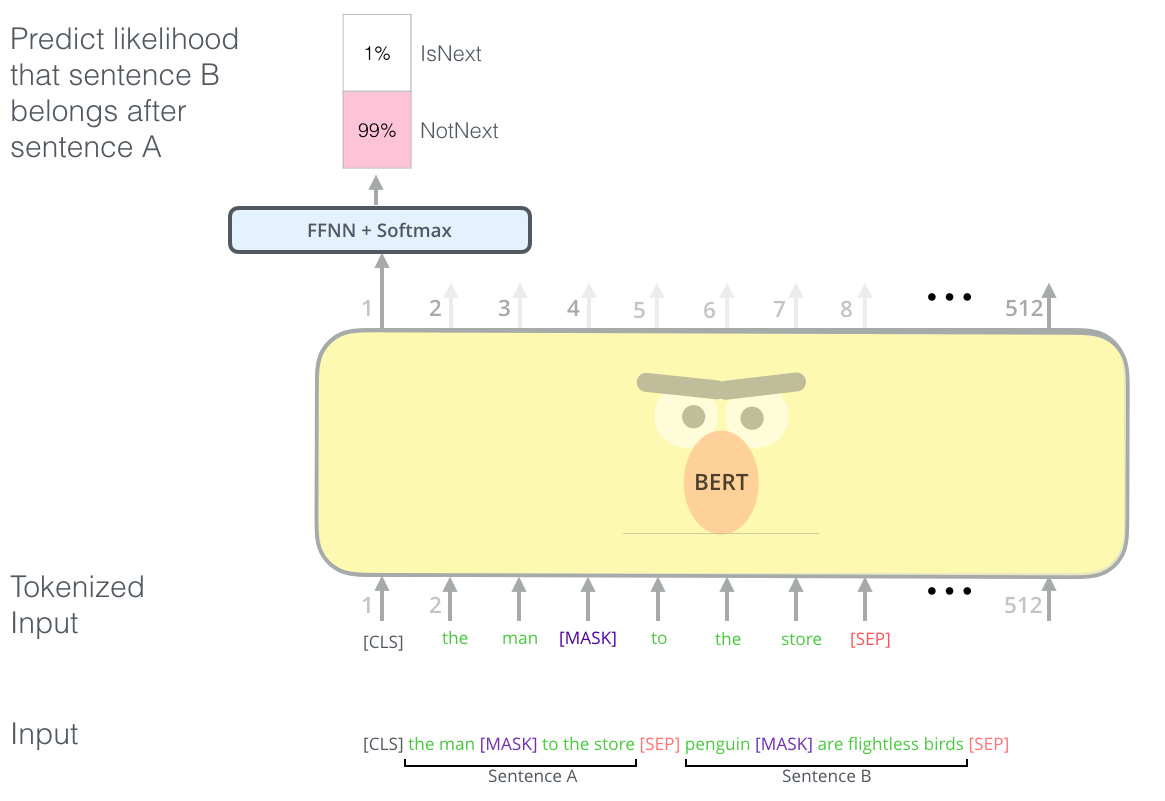
MLM으로 BERT를 학습시킨 후, 두번째로 two-sentence classification 테스크를 이용해 BERT 를 pre-train 합니다. 위의 이미지에는 실제 BERT와는 달리 단어 분리 (tokenization)이 매우 간단하게 표현되어 있습니다. 실제로 BERT는 단어가 아닌 WordPieces라는 더 작은 단위의 token으로 입력 단어들을 쪼갭니다. The second task BERT is pre-trained on is a two-sentence classification task. The tokenization is oversimplified in this graphic as BERT actually uses WordPieces as tokens rather than words — so some words are broken down into smaller chunks.
목표 Task에 맞게 모델 학습시키기
BERT의 논문에서는 여러가지 테스크들에서 어떻게 BERT 모델을 활용할 수 있는지 보여주고 있습니다. downstream 테스크들을 크게 네가지로 나누어 설명하고 있는 아래의 그림을 참고하세요. The BERT paper shows a number of ways to use BERT for different tasks.
BERT 로 feature extraction 하기
BERT를 활용하는 방법에 fine-tuning만 있는 것은 아닙니다. ELMo와 마찬가지로, pre-train된 BERT를 이용해서 contextualized word embedding을 뽑아낼 수 있습니다. 그리고 그 word embedding을 당신의 모델에 단어의 feature으로서 넣어주면 되는거죠. 놀랍게도 이러한 방법으로 named-entity recognition 모델을 학습시켜 보았을 때 fine-tuning에 비해 크게 뒤져지지 않음을 논문에서 보여주고 있습니다. The fine-tuning approach isn’t the only way to use BERT. Just like ELMo, you can use the pre-trained BERT to create contextualized word embeddings. Then you can feed these embeddings to your existing model – a process the paper shows yield results not far behind fine-tuning BERT on a task such as named-entity recognition.
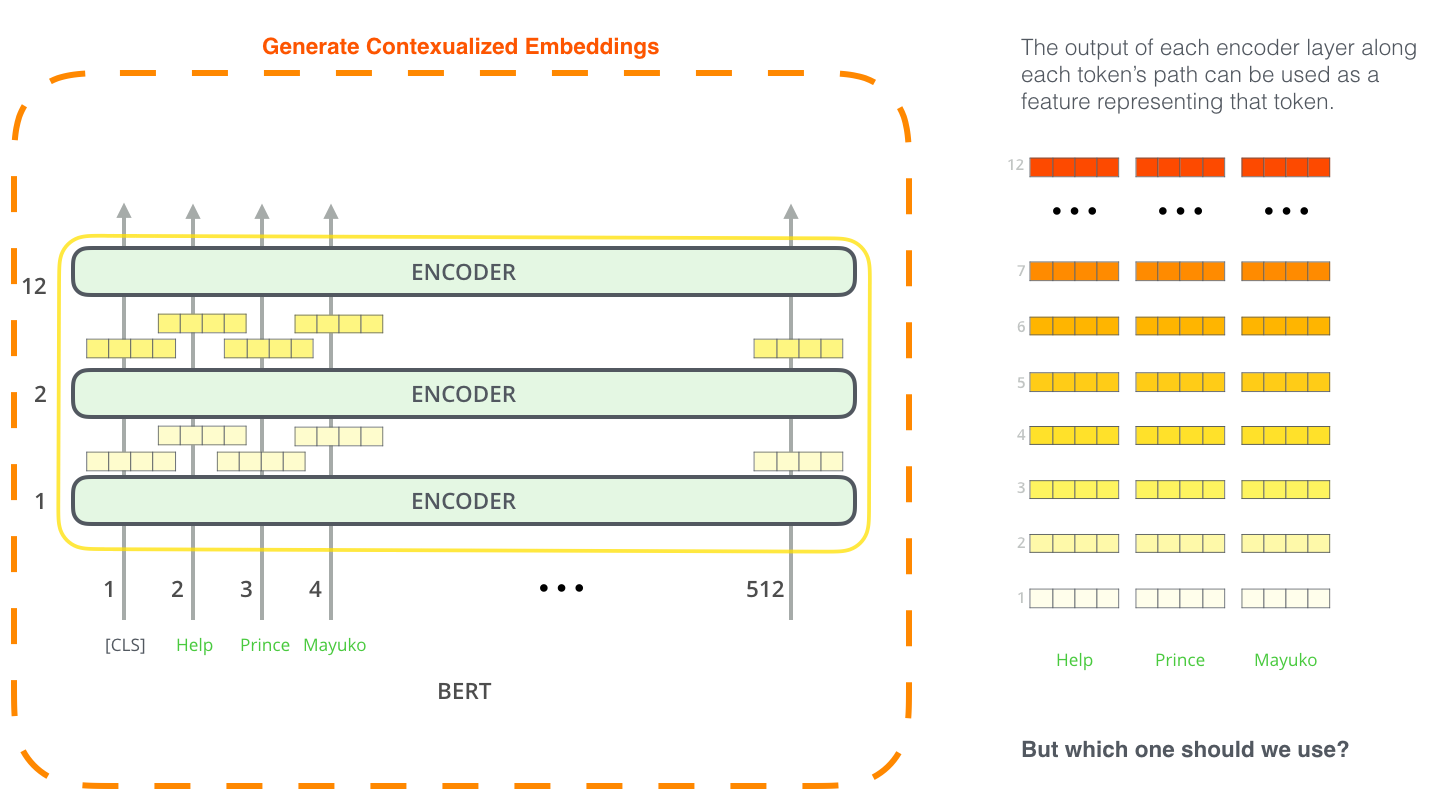
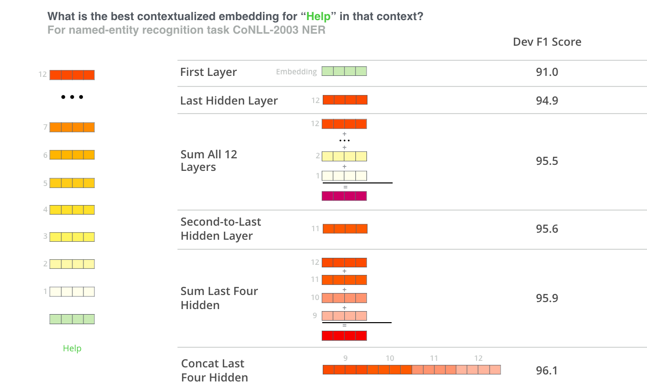
그렇다면 BERT에서 어떻게 contextualized embedding을 뽑는게 가장 좋을까요? 그것은 어떤 테스크냐에 따라 대답이 달라진다고 생각합니다. 논문에서는 여섯가지의 방법들을 실험해보았는데요, NER 테스크에서 fine-tune한 모델의 성능은 96.4 였다는 사실을 감안하고 아래의 결과를 한번 보시죠: Which vector works best as a contextualized embedding? I would think it depends on the task. The paper examines six choices (Compared to the fine-tuned model which achieved a score of 96.4):
BERT 직접 (간단히) 테스트 해보기
BERT를 테스트 해보는 가장 좋은 방법은 Cloud TPUs로 BERT FineTuning 하기 라는 Google Colab에 있는 주피터 노트북을 써보는 것입니다. Cloud TPU를 한번도 써보신 적이 없으시다면 이 노트북이 TPU를 써보는 좋은 기회가 될 수도 있겠네요. 하지만, 위의 노트북에서 BERT 코드는 TPU 뿐만 아니라 CPU와 GPU에서도 돌아가니 겁내지 마세요! The best way to try out BERT is through the BERT FineTuning with Cloud TPUs notebook hosted on Google Colab. If you’ve never used Cloud TPUs before, this is also a good starting point to try them as well as the BERT code works on TPUs, CPUs and GPUs as well.
그 다음으로 해볼 수 있는 것은 BERT의 공식 repo에 가서 직접 코드를 읽어보는 것입니다: The next step would be to look at the code in the BERT repo:
- 실제 모델은 modeling.py 파일에서 (
BertModel 클래스)로 구현되어 있습니다. 사실 기존의 트랜스포머 encoder와 거의 똑같습니다. - run_classifier.py 코드에서는 fine-tuning 하는 과정을 볼 수 있습니다. 이 예제에서는 supervised 분류 (classification)모델을 위해서 따로 층을 하나 마지막에 만듭니다. 만약에 유사하게 본인의 분류 모델을 만들고 싶으시다면
create_model()함수를 참고하세요. - 여러가지 버전의 pre-train된 모델들을 다운받으실 수 있습니다. 대표적으로 BERT Base와 BERT Large 가 있구요, 또한 영어 외에도 중국어, 프랑스어 등 위키피디아의 102개의 다른 언어들을 이용해서 학습시킨 모델들도 있습니다.
- BERT는 단어를 token으로 사용하지 않습니다. 단어 대신 WordPieces 라는 더 작은 단위를 이용하는데요, tokenization.py에서 보면 입력 문장을 BERT가 입력 받을 수 있는 WordPieces들로 나누어주는 tokenizer가 구현되어 있습니다.
-The model is constructed in modeling.py (
class BertModel) and is pretty much identical to a vanilla Transformer encoder. -run_classifier.py is an example of the fine-tuning process. It also constructs the classification layer for the supervised model. If you want to construct your own classifier, check out thecreate_model()method in that file. -Several pre-trained models are available for download. These span BERT Base and BERT Large, as well as languages such as English, Chinese, and a multi-lingual model covering 102 languages trained on wikipedia. -BERT doesn’t look at words as tokens. Rather, it looks at WordPieces. tokenization.py is the tokenizer that would turns your words into wordPieces appropriate for BERT.
또 다른 좋은 repo로는 huggigface에서 작성한 PyTorch implementation of BERT가 있습니다. AllenNLP 라이브러리들은 이 repo를 바탕으로 해서 BERT embeddings을 다른 모델들에 적용할 수 있도록 하고 있습니다. You can also check out the PyTorch implementation of BERT. The AllenNLP library uses this implementation to allow using BERT embeddings with any model.
도움 주신 분들
초반의 원고에 피드백을 준 Jacob Devlin, Matt Gardner, Kenton Lee, Mark Neumann, Matthew Peters에게 감사를 전합니다. Thanks to Jacob Devlin, Matt Gardner, Kenton Lee, Mark Neumann, and Matthew Peters for providing feedback on earlier drafts of this post.