The Illustrated Transformer
저번 글에서 다뤘던 attention seq2seq 모델에 이어, attention 을 활용한 또 다른 모델인 Transformer 모델에 대해 얘기해보려 합니다. 2017 NIPS에서 Google이 소개했던 Transformer는 NLP 학계에서 정말 큰 주목을 끌었는데요, 어떻게 보면 기존의 CNN 과 RNN 이 주를 이뤘던 연구들에서 벗어나 아예 새로운 모델을 제안했기 때문이지 않을까 싶습니다. 실제로 적용했을 때 최근 연구에 비해 큰 성능 향상을 보여줬기 때문이기도 하고요.
이 모델의 핵심을 정리해보자면, multi-head self-attention을 이용해 sequential computation 을 줄여 더 많은 부분을 병렬처리가 가능하게 만들면서 동시에 더 많은 단어들 간 dependency를 모델링 한다는 것입니다. 이하 글에서 이 self-attention에 대해서 더 자세히 알아보도록 하겠습니다. 아래의 글은 저번 attention seq2seq 모델과 동일한 블로그 by Jay Alammar에서 허락을 받고 가져온 글이며, 원문은 본 링크 에서 확인하실 수 있습니다.
아래의 번역 글은 마우스를 올리시면 (모바일의 경우 터치) 원문을 확인하실 수 있습니다. 혹시 번역에 심각한 오류 혹은 오탈자를 확인하신다면 밑의 Disqus 댓글 창에 남겨주시면 감사하겠습니다.
(이하 본문)
Transformer 모델의 시각화 by Jay Alammar
저번 글 에서 attention 에 대해 알아보았습니다 – 현대 딥러닝 모델들에서 아주 넓게 이용되고 있는 메소드죠. Attention 은 신경망 기계 번역과 그 응용 분야들의 성능을 향상시키는데 도움이 된 컨셉입니다. 이번 글에서는 우리는 이 attention 을 활용한 모델인 Transformer에 대해 다룰 것입니다 – attention 을 학습하여 그를 통해 학습 속도를 크게 향상시킨 모델이죠. 이 Transformer 모델은 몇몇의 테스크에서 기존의 seq2seq를 활용한 구글 신경망 번역 시스템 보다 좋은 성능을 보입니다. 하지만 이것의 가장 큰 장점은 병렬처리에 관한 부분입니다. Google Cloud는 이제 그들의 Cloud TPU를 쓸 때 Transfomer 모델을 기준으로 쓸 것을 추천하고 있습니다. 이제 한 번 이 모델이 어떻게 작동하는지 부분 부분 나누어 알아보겠습니다. In the previous post, we looked at Attention – a ubiquitous method in modern deep learning models. Attention is a concept that helped improve the performance of neural machine translation applications. In this post, we will look at The Transformer – a model that uses attention to boost the speed with which these models can be trained. The Transformers outperforms the Google Neural Machine Translation model in specific tasks. The biggest benefit, however, comes from how The Transformer lends itself to parallelization. It is in fact Google Cloud’s recommendation to use The Transformer as a reference model to use their Cloud TPU offering. So let’s try to break the model apart and look at how it functions.
Transformer 은 Attention is All You Need이라는 논문을 통해 처음 발표되었습니다. 이 모델의 TensorFlow 구현은 Tensor2Tensor package의 일부로서 현재 확인할 수 있습니다. Harvard NLP 그룹에서 나온 guide annotating the paper with PyTorch implementation라는 글은 PyTorch 구현과 함께 모델에 대한 자세한 설명을 담고 있으니 확인해보셔도 좋을 것 같습니다. 본 글에서는 이미 모든 컨셉들에 대해 깊이 알고 있지 않아도 이해할 수 있도록, 많은 것들을 최대한 단순화한 채로 여러 가지 개념들을 하나씩 하나씩 설명해보도록 하겠습니다. The Transformer was proposed in the paper Attention is All You Need. A TensorFlow implementation of it is available as a part of the Tensor2Tensor package. Harvard’s NLP group created a guide annotating the paper with PyTorch implementation. In this post, we will attempt to oversimplify things a bit and introduce the concepts one by one to hopefully make it easier to understand to people without in-depth knowledge of the subject matter.
개괄적인 수준의 설명
A High-Level Look
먼저 모델의 자세한 부분을 무시하고, 이를 하나의 black box라고 보겠습니다. 기계 번역의 경우를 생각해본다면, 모델은 어떤 한 언어로 된 하나의 문장을 입력으로 받아 다른 언어로 된 번역을 출력으로 내놓을 것입니다. Let’s begin by looking at the model as a single black box. In a machine translation application, it would take a sentence in one language, and output its translation in another.
그 black box를 열어 보게 되면 우리는 encoding 부분, decoding 부분, 그리고 그 사이를 이어주는 connection들을 보게 됩니다. Popping open that Optimus Prime goodness, we see an encoding component, a decoding component, and connections between them.
encoding 부분은 여러 개의 encoder 을 쌓아 올려 만든 것입니다 (논문에서는 6개를 쌓았다고 합니다만 꼭 6개를 쌓아야 하는 것은 아니고 각자의 세팅에 맞게 얼마든지 변경하여 실험할 수 있습니다). decoding 부분은 encoding 부분과 동일한 개수만큼의 decoder 을 쌓은 것을 말합니다. The encoding component is a stack of encoders (the paper stacks six of them on top of each other – there’s nothing magical about the number six, one can definitely experiment with other arrangements). The decoding component is a stack of decoders of the same number.
encoder 들은 모두 정확히 똑같은 구조를 가지고 있습니다 (그러나 그들 간에 같은 weight을 공유하진 않습니다). 하나의 encoder를 나눠보면 아래와 같이 두 개의 sub-layer으로 구성되어 있습니다: The encoders are all identical in structure (yet they do not share weights). Each one is broken down into two sub-layers:
인코더에 들어온 입력은 일단 먼저 self-attention layer을 지나가게 됩니다 – 이 layer 은 encoder가 하나의 특정한 단어를 encode 하기 위해서 입력 내의 모든 다른 단어들과의 관계를 살펴봅니다. 이 self-attention 층에 대해서는 조금 있다가 더 자세히 알아보도록 하겠습니다. The encoder’s inputs first flow through a self-attention layer – a layer that helps the encoder look at other words in the input sentence as it encodes a specific word. We’ll look closer at self-attention later in the post.
입력이 self-attention 층을 통과하여 나온 출력은 다시 feed-forward 신경망으로 들어가게 됩니다. 똑같은 feed-forward 신경망이 각 위치의 단어마다 독립적으로 적용돼 출력을 만듭니다. The outputs of the self-attention layer are fed to a feed-forward neural network. The exact same feed-forward network is independently applied to each position.
decoder 또한 encoder에 있는 두 layer 모두를 가지고 있습니다. 그러나 그 두 층 사이에 seq2seq 모델의 attention 과 비슷한 encoder-decoder attention 이 포함되어 있습니다. 이는 decoder가 입력 문장 중에서 각 타임 스텝에서 가장 관련 있는 부분에 집중할 수 있도록 해줍니다. The decoder has both those layers, but between them is an attention layer that helps the decoder focus on relevant parts of the input sentence (similar what attention does in seq2seq models).
벡터들을 기준으로 그림 그려보기
Bringing The Tensors Into The Picture
이제 우리는 Transformer 모델의 주요 부분들에 대해서 다 알아보았는데요, 이제 입력으로 들어와서 출력이 될 때까지 이 부분들 사이를 지나가며 변환될 벡터/텐서들을 기준으로 모델을 살펴보도록 하겠습니다. Now that we’ve seen the major components of the model, let’s start to look at the various vectors/tensors and how they flow between these components to turn the input of a trained model into an output.
현대에 들어 대부분 NLP 관련 모델에서 그러듯, 먼저 입력 단어들을 embedding 알고리즘를 이용해 벡터로 바꾸는 것부터 해야 합니다. As is the case in NLP applications in general, we begin by turning each input word into a vector using an embedding algorithm.
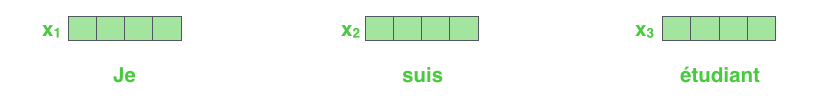
각 단어들은 크기 512의 벡터 하나로 embed 됩니다. 우리는 이 변환된 벡터들을 위와 같은 간단한 박스로 나타내겠습니다. Each word is embedded into a vector of size 512. We’ll represent those vectors with these simple boxes.
이 embedding은 가장 밑단의 encoder 에서만 일어납니다. 이렇게 되면 이제 우리는 이렇게 뭉뚱그려 표현할 수 있게 됩니다; 모든 encoder 들은 크기 512의 벡터의 리스트를 입력으로 받습니다 – 이 벡터는 가장 밑단의 encoder의 경우에는 word embedding이 될 것이고, 다른 encoder들에서는 바로 전의 encoder의 출력일 것입니다. 이 벡터 리스트의 사이즈는 hyperparameter으로 우리가 마음대로 정할 수 있습니다 – 가장 간단하게 생각한다면 우리의 학습 데이터 셋에서 가장 긴 문장의 길이로 둘 수 있습니다. The embedding only happens in the bottom-most encoder. The abstraction that is common to all the encoders is that they receive a list of vectors each of the size 512 – In the bottom encoder that would be the word embeddings, but in other encoders, it would be the output of the encoder that’s directly below. The size of this list is hyperparameter we can set – basically it would be the length of the longest sentence in our training dataset.
입력 문장의 단어들을 embedding 한 후에, 각 단어에 해당하는 벡터들은 encoder 내의 두 개의 sub-layer으로 들어가게 됩니다. After embedding the words in our input sequence, each of them flows through each of the two layers of the encoder.
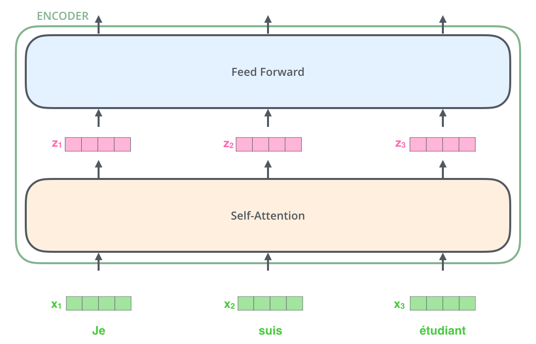
여기서 우리는 각 위치에 있는 각 단어가 그만의 path를 통해 encoder에서 흘러간다는 Transformer 모델의 주요 성질을 볼 수 있습니다. Self-attention 층에서 이 위치에 따른 path들 사이에 다 dependency가 있습니다. 반면 feed-forward 층은 이런 dependency가 없기 때문에 feed-forward layer 내의 이 다양한 path 들은 병렬처리될 수 있습니다. Here we begin to see one key property of the Transformer, which is that the word in each position flows through its own path in the encoder. There are dependencies between these paths in the self-attention layer. The feed-forward layer does not have those dependencies, however, and thus the various paths can be executed in parallel while flowing through the feed-forward layer.
이제 우리는 이 예시를 조금 더 짧은 문장으로 바꾸어 encoder의 각 sub-layer에서 무슨 일이 일어나는지를 자세히 보도록 하겠습니다. Next, we’ll switch up the example to a shorter sentence and we’ll look at what happens in each sub-layer of the encoder.
이제 Encoding을 해봅시다!
Now We’re Encoding!
앞서 설명한 것과 같이, encoder는 입력으로 벡터들의 리스트를 받습니다. 이 리스트를 먼저 self-attention layer에, 그다음으로 feed-forward 신경망에 통과시키고 그 결과물을 그다음 encoder에게 전달합니다. As we’ve mentioned already, an encoder receives a list of vectors as input. It processes this list by passing these vectors into a ‘self-attention’ layer, then into a feed-forward neural network, then sends out the output upwards to the next encoder.
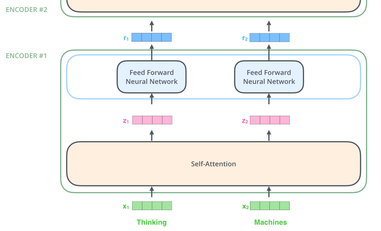
각 위치의 단어들은 각각 다른 self-encoding 과정을 거칩니다. 그다음으로는 모두에게 같은 과정인 feed-forward 신경망을 거칩니다. The word at each position passes through a self-encoding process. Then, they each pass through a feed-forward neural network – the exact same network with each vector flowing through it separately.
크게 크게 살펴보는 Self-Attention
Self-Attention at a High Level
비록 현재까지 제가 self-attention이라는 단어를 반복적으로 쓰고 있긴 하지만 이것이 모두가 알고 있을만한 개념이라는 뜻은 아닙니다. 저 또한 개인적으로 “Attention is All You Need” 논문을 읽기 전에는 이 개념에 대해서 들어본 적조차 없었습니다. 이제 이 개념이 작동하는지 자세히 알아보도록 하겠습니다. Don’t be fooled by me throwing around the word “self-attention” like it’s a concept everyone should be familiar with. I had personally never came across the concept until reading the Attention is All You Need paper. Let us distill how it works.
다음 문장을 우리가 번역하고 싶은 문장이라고 치겠습니다:
“그 동물은 길을 건너지 않았다 왜냐하면 그것은 너무 피곤했기 때문이다”
The animal didn’t cross the street because it was too tired
이 문장에서 “그것” 이 가리키는 것은 무엇일까요? “그것”은 길을 말하는 것일까요 아니면 동물을 말하는 것일까요? 사람에게는 이것이 너무나도 간단한 질문이지만 신경망 모델에게는 그렇게 간단하지만은 않은 문제입니다. What does “it” in this sentence refer to? Is it referring to the street or to the animal? It’s a simple question to a human, but not as simple to an algorithm.
모델이 “그것은”이라는 단어를 처리할 때, 모델은 self-attention 을 이용하여 “그것”과 “동물”을 연결할 수 있습니다. When the model is processing the word “it”, self-attention allows it to associate “it” with “animal”.
모델이 입력 문장 내의 각 단어를 처리해 나감에 따라, self-attention은 입력 문장 내의 다른 위치에 있는 단어들을 보고 거기서 힌트를 받아 현재 타겟 위치의 단어를 더 잘 encoding 할 수 있습니다. As the model processes each word (each position in the input sequence), self attention allows it to look at other positions in the input sequence for clues that can help lead to a better encoding for this word.
만약 RNN에 익숙하시다면, RNN이 hidden state를 유지하고 업데이트함으로써 현재 처리 중인 단어에 어떻게 과거의 단어들에서 나온 맥락을 연관시키는지 생각해보세요. 그와 동일하게 Transformer에게는 이 self-attention이 현재 처리 중인 단어에 다른 연관 있는 단어들의 맥락을 불어 넣어주는 method입니다. If you’re familiar with RNNs, think of how maintaining a hidden state allows an RNN to incorporate its representation of previous words/vectors it has processed with the current one it’s processing. Self-attention is the method the Transformer uses to bake the “understanding” of other relevant words into the one we’re currently processing.
가장 윗단에 있는 encoder #5에서 “그것”이라는 단어를 encoding 할 때, attention 메커니즘은 입력의 여러 단어들 중에서 “그 동물”이라는 단어에 집중하고 이 단어의 의미 중 일부를 “그것”이라는 단어를 encoding 할 때 이용합니다. As we are encoding the word “it” in encoder #5 (the top encoder in the stack), part of the attention mechanism was focusing on “The Animal”, and baked a part of its representation into the encoding of “it”.
이 Tensor2Tensor 노트북 에서는 Transformer 모델을 불러와서 인터랙티브한 시각화를 통해 여러 가지 사항들을 직접 실험해보실 수 있으니 한 번 확인해보세요. Be sure to check out the Tensor2Tensor notebook where you can load a Transformer model, and examine it using this interactive visualization.
Self-Attention 을 더 자세히 보겠습니다.
Self-Attention in Detail
이번 섹션에서는 먼저 여러 가지 벡터들을 통해서 어떻게 self-attention 을 계산할 수 있는지 보겠습니다. 그 후 행렬을 이용해서 이것이 실제로 어떻게 구현돼 있는지 확인하겠습니다. Let’s first look at how to calculate self-attention using vectors, then proceed to look at how it’s actually implemented – using matrices.
self-attention 계산의 가장 첫 단계는 encoder에 입력된 벡터들 (이 경우에서는 각 단어의 embedding 벡터입니다)에게서 부터 각 3개의 벡터를 만들어내는 일입니다. 우리는 각 단어에 대해서 Query 벡터, Key 벡터, 그리고 Value 벡터를 생성합니다. 이 벡터들은 입력 벡터에 대해서 세 개의 학습 가능한 행렬들을 각각 곱함으로써 만들어집니다. The first step in calculating self-attention is to create three vectors from each of the encoder’s input vectors (in this case, the embedding of each word). So for each word, we create a Query vector, a Key vector, and a Value vector. These vectors are created by multiplying the embedding by three matrices that we trained during the training process.
여기서 한가지 짚고 넘어갈 것은 이 새로운 벡터들이 기존의 벡터들 보다 더 작은 사이즈를 가진다는 것입니다. 기존의 입력 벡터들은 크기가 512인 반면 이 새로운 벡터들은 크기가 64입니다. 그러나 그들이 꼭 이렇게 더 작아야만 하는 것은 아니며, 이것은 그저 multi-head attention의 계산 복잡도를 일정하게 만들고자 내린 구조적인 선택일 뿐입니다. Notice that these new vectors are smaller in dimension than the embedding vector. Their dimensionality is 64, while the embedding and encoder input/output vectors have dimensionality of 512. They don’t HAVE to be smaller, this is an architecture choice to make the computation of multiheaded attention (mostly) constant.
x1를 weight 행렬인 WQ로 곱하는 것은 현재 단어와 연관된 query 벡터인 q1를 생성합니다. 같은 방법으로 우리는 입력 문장에 있는 각 단어에 대한 query, key, value 벡터를 만들 수 있습니다. Multiplying x1 by the WQ weight matrix produces q1, the “query” vector associated with that word. We end up creating a “query”, a “key”, and a “value” projection of each word in the input sentence.
그렇다면 정확히 이 query, key, value 벡터란 무엇을 의미하는 것일까요? What are the “query”, “key”, and “value” vectors?
그것은 attention 에 대해서 생각하고 계산하려할 때 도움이 되는 추상적인 개념입니다. 이제 곧 다루게 될 테지만 어떻게 attention 이 실제로 계산되는지를 알게 되면, 자연스럽게 이 세 개의 벡터들이 어떤 역할을 하는지 알 수 있게 됩니다. They’re abstractions that are useful for calculating and thinking about attention. Once you proceed with reading how attention is calculated below, you’ll know pretty much all you need to know about the role each of these vectors plays.
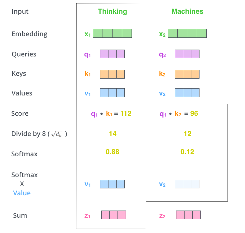
self-attention 계산의 두 번째 스텝은 점수를 계산하는 것입니다. 아래 예시의 첫 번째 단어인 “Thinking”에 대해서 self-attention 을 계산한다고 하겠습니다. 우리는 이 단어와 입력 문장 속의 다른 모든 단어들에 대해서 각각 점수를 계산하여야 합니다. 이 점수는 현재 위치의 이 단어를 encode 할 때 다른 단어들에 대해서 얼마나 집중을 해야 할지를 결정합니다. The second step in calculating self-attention is to calculate a score. Say we’re calculating the self-attention for the first word in this example, “Thinking”. We need to score each word of the input sentence against this word. The score determines how much focus to place on other parts of the input sentence as we encode a word at a certain position.
점수는 현재 단어의 query vector와 점수를 매기려 하는 다른 위치에 있는 단어의 key vector의 내적으로 계산됩니다. 다시 말해, 우리가 위치 #1에 있는 단어에 대해서 self-attention 을 계산한다 했을 때, 첫 번째 점수는 q1과 k1의 내적일 것입니다. 그리고 동일하게 두 번째 점수는 q1과 k2의 내적일 것입니다. The score is calculated by taking the dot product of the query vector with the key vector of the respective word we’re scoring. So if we’re processing the self-attention for the word in position #1, the first score would be the dot product of q1 and k1. The second score would be the dot product of q1 and k2.
세 번째와 네 번째 단계는 이 점수들을 8로 나누는 것입니다. 이 8이란 숫자는 key 벡터의 사이즈인 64의 제곱 근이라는 식으로 계산이 된 것입니다. 이 나눗셈을 통해 우리는 더 안정적인 gradient를 가지게 됩니다. 그리고 난 다음 이 값을 softmax 계산을 통과시켜 모든 점수들을 양수로 만들고 그 합을 1으로 만들어 줍니다. The third and forth steps are to divide the scores by 8 (the square root of the dimension of the key vectors used in the paper – 64. This leads to having more stable gradients. There could be other possible values here, but this is the default), then pass the result through a softmax operation. Softmax normalizes the scores so they’re all positive and add up to 1.
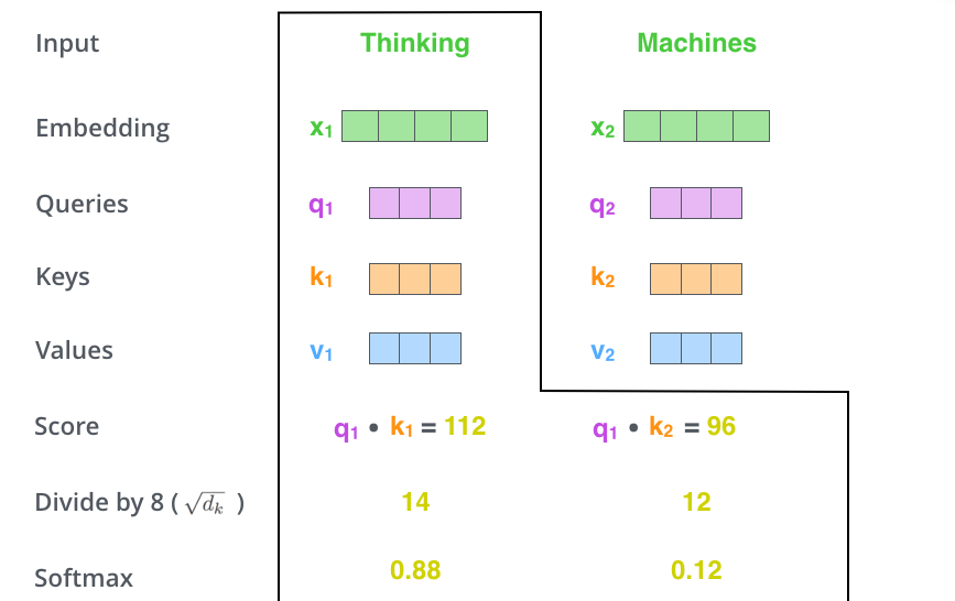
이 softmax 점수는 현재 위치의 단어의 encoding에 있어서 얼마나 각 단어들의 표현이 들어갈 것인지를 결정합니다. 당연하게 현재 위치의 단어가 가장 높은 점수를 가지며 가장 많은 부분을 차지하게 되겠지만, 가끔은 현재 단어에 관련이 있는 다른 단어에 대한 정보가 들어가는 것이 도움이 됩니다. This softmax score determines how much how much each word will be expressed at this position. Clearly the word at this position will have the highest softmax score, but sometimes it’s useful to attend to another word that is relevant to the current word.
다섯 번째 단계는 이제 입력의 각 단어들의 value 벡터에 이 점수를 곱하는 것입니다. 이것을 하는 이유는 우리가 집중을 하고 싶은 관련이 있는 단어들은 그래도 남겨두고, 관련이 없는 단어들은 0.001 과 같은 작은 숫자 (점수)를 곱해 없애버리기 위함입니다. The fifth step is to multiply each value vector by the softmax score (in preparation to sum them up). The intuition here is to keep intact the values of the word(s) we want to focus on, and drown-out irrelevant words (by multiplying them by tiny numbers like 0.001, for example).
마지막 여섯 번째 단계는 이 점수로 곱해진 weighted value 벡터들을 다 합해 버리는 것입니다. 이 단계의 출력이 바로 현재 위치에 대한 self-attention layer의 출력이 됩니다. The sixth step is to sum up the weighted value vectors. This produces the output of the self-attention layer at this position (for the first word).
이 여섯 가지 과정이 바로 self-attention의 계산 과정입니다. 우리는 이 결과로 나온 벡터를 feed-forward 신경망으로 보내게 됩니다. 그러나 실제 구현에서는 빠른 속도를 위해 이 모든 과정들이 벡터가 아닌 행렬의 형태로 진행됩니다. 우리는 이때까지 각 단어 레벨에서의 계산과 그 이유에 대해서 얘기해봤다면, 이제 이 행렬 레벨의 계산을 살펴보도록 하겠습니다. That concludes the self-attention calculation. The resulting vector is one we can send along to the feed-forward neural network. In the actual implementation, however, this calculation is done in matrix form for faster processing. So let’s look at that now that we’ve seen the intuition of the calculation on the word level.
Self-attention 의 행렬 계산
Matrix Calculation of Self-Attention
가장 첫 스텝은 입력 문장에 대해서 Query, Key, Value 행렬들을 계산하는 것입니다. 이를 위해 우리는 우리의 입력 벡터들 (혹은 embedding 벡터들)을 하나의 행렬 X로 쌓아 올리고, 그것을 우리가 학습할 weight 행렬들인 WQ, WK, WV 로 곱합니다. The first step is to calculate the Query, Key, and Value matrices. We do that by packing our embeddings into a matrix X, and multiplying it by the weight matrices we’ve trained (WQ, WK, WV).
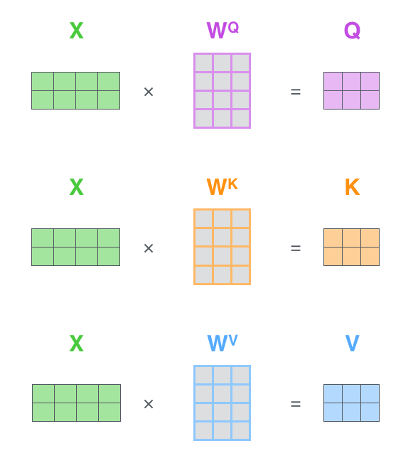
행렬 X의 각 행은 입력 문장의 각 단어에 해당합니다. 우리는 여기서 다시 한번 embedding 벡터들 (크기 512, 그림에서는 4)과 query/key/value 벡터들 (크기 64, 그림에서는 3) 간의 크기 차이를 볼 수 있습니다. Every row in the X matrix corresponds to a word in the input sentence. We again see the difference in size of the embedding vector (512, or 4 boxes in the figure), and the q/k/v vectors (64, or 3 boxes in the figure)
마지막으로, 우리는 현재 행렬을 이용하고 있으므로 앞서 설명했던 self-attention 계산 단계 2부터 6까지를 하나의 식으로 압축할 수 있습니다. Finally, since we’re dealing with matrices, we can condense steps two through six in one formula to calculate the outputs of the self-attention layer.
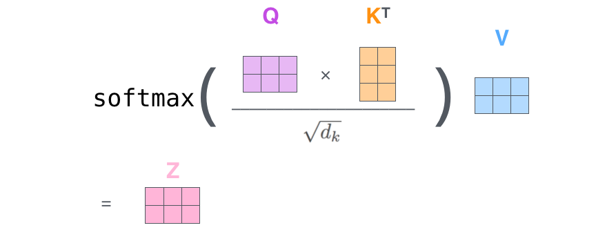
행렬 형태로 표현한 self-attention 계산 The self-attention calculation in matrix form
The Beast With Many Heads
The Beast With Many Heads
본 논문은 이 self-attention layer에다 “multi-headed” attention이라는 메커니즘을 더해 더욱더 이를 개선합니다. 이것은 두 가지 방법으로 attention layer의 성능을 향상시킵니다: The paper further refined the self-attention layer by adding a mechanism called “multi-headed” attention. This improves the performance of the attention layer in two ways:
- 모델이 다른 위치에 집중하는 능력을 확장시킵니다. 위의 예시에서는 z1 이 모든 다른 단어들의 encoding 을 조금씩 포함했지만, 사실 이것은 실제 자기 자신에게만 높은 점수를 줘 자신만을 포함해도 됐을 것입니다. 이것은 “그 동물은 길을 건너지 않았다 왜냐하면 그것은 너무 피곤했기 때문이다” 과 같은 문장을 번역할 때 “그것”이 무엇을 가리키는지에 대해 알아낼 때 유용합니다.
- attention layer 가 여러 개의 “representation 공간”을 가지게 해줍니다. 계속해서 보겠지만, multi-headed attention을 이용함으로써 우리는 여러 개의 query/key/value weight 행렬들을 가지게 됩니다 (논문에서 제안된 구조는 8개의 attention heads를 가지므로 우리는 각 encoder/decoder마다 이런 8개의 세트를 가지게 되는 것입니다). 이 각각의 query/key/value set는 랜덤으로 초기화되어 학습됩니다. 학습이 된 후 각각의 세트는 입력 벡터들에 곱해져 벡터들을 각 목적에 맞게 투영시키게 됩니다. 이러한 세트가 여러개 있다는 것은 각 벡터들을 각각 다른 representation 공간으로 나타낸 다는 것을 의미합니다. 1.It expands the model’s ability to focus on different positions. Yes, in the example above, z1 contains a little bit of every other encoding, but it could be dominated by the the actual word itself. It would be useful if we’re translating a sentence like “The animal didn’t cross the street because it was too tired”, we would want to know which word “it” refers to. 2.It gives the attention layer multiple “representation subspaces”. As we’ll see next, with multi-headed attention we have not only one, but multiple sets of Query/Key/Value weight matrices (the Transformer uses eight attention heads, so we end up with eight sets for each encoder/decoder). Each of these sets is randomly initialized. Then, after training, each set is used to project the input embeddings (or vectors from lower encoders/decoders) into a different representation subspace.
multi-headed attention을 이용하기 위해서 우리는 각 head를 위해서 각각의 다른 query/key/value weight 행렬들을 모델에 가지게 됩니다. 이전에 설명한 것과 같이 우리는 입력 벡터들의 모음인 행렬 X를 WQ/WK/WV 행렬들로 곱해 각 head에 대한 Q/K/V 행렬들을 생성합니다. With multi-headed attention, we maintain separate Q/K/V weight matrices for each head resulting in different Q/K/V matrices. As we did before, we multiply X by the WQ/WK/WV matrices to produce Q/K/V matrices.
위에 설명했던 대로 같은 self-attention 계산 과정을 8개의 다른 weight 행렬들에 대해 8번 거치게 되면, 우리는 8개의 서로 다른 Z 행렬을 가지게 됩니다. If we do the same self-attention calculation we outlined above, just eight different times with different weight matrices, we end up with eight different Z matrices
그러나 문제는 이 8개의 행렬을 바로 feed-forward layer으로 보낼 수 없다는 것입니다. feed-forward layer 은 한 위치에 대해 오직 한 개의 행렬만을 input으로 받을 수 있습니다. 그러므로 우리는 이 8개의 행렬을 하나의 행렬로 합치는 방법을 고안해 내야 합니다. This leaves us with a bit of a challenge. The feed-forward layer is not expecting eight matrices – it’s expecting a single matrix (a vector for each word). So we need a way to condense these eight down into a single matrix.
어떻게 할 수 있을까요? 간단합니다. 일단 모두 이어 붙여서 하나의 행렬로 만들어버리고, 그다음 하나의 또 다른 weight 행렬인 W0을 곱해버립니다. How do we do that? We concat the matrices then multiple them by an additional weights matrix WO.
사실상 multi-headed self-attention 은 이게 다입니다. 비록 여러 개의 행렬들이 등장하긴 했지만요. 이제 이 모든 것을 하나의 그림으로 표현해서 모든 과정을 한눈에 정리해보도록 하겠습니다. That’s pretty much all there is to multi-headed self-attention. It’s quite a handful of matrices, I realize. Let me try to put them all in one visual so we can look at them in one place
여기까지 attention heads에 대해서 설명해 보았는데요, 이제 다시 우리의 예제 문장을 multi-head attention 과 함께 보도록 하겠습니다. 그중에서도 특히 “그것” 이란 단어를 encode 할 때 여러 개의 attention 이 각각 어디에 집중하는지를 보도록 하겠습니다; Now that we have touched upon attention heads, let’s revisit our example from before to see where the different attention heads are focusing as we encode the word “it” in our example sentence:
우리가 “그것” 이란 단어를 encode 할 때, 주황색의 attention head 는 “그 동물”에 가장 집중하고 있는 반면 초록색의 head는 “피곤”이라는 단어에 집중을 하고 있습니다. 모델은 이 두 개의 attention head를 이용하여 “동물”과 “피곤” 두 단어 모두에 대한 representation 을 “그것”의 representation에 포함시킬 수 있습니다. As we encode the word “it”, one attention head is focusing most on “the animal”, while another is focusing on “tired” – in a sense, the model’s representation of the word “it” bakes in some of the representation of both “animal” and “tired”.
그러나 이 모든 attention head들을 하나의 그림으로 표현하면, 이제 attention의 의미는 해석하기가 어려워집니다: If we add all the attention heads to the picture, however, things can be harder to interpret:
Positional Encoding 을 이용해서 시퀀스의 순서 나타내기
Representing The Order of The Sequence Using Positional Encoding
우리가 이때까지 설명해온 Transformer 모델에서 한가지 부족한 부분은 이 모델이 입력 문장에서 단어들의 순서에 대해서 고려하고 있지 않다는 점입니다. One thing that’s missing from the model as we have described it so far is a way to account for the order of the words in the input sequence.
이것을 추가하기 위해서, Transformer 모델은 각각의 입력 embedding에 “positional encoding”이라고 불리는 하나의 벡터를 추가합니다. 이 벡터들은 모델이 학습하는 특정한 패턴을 따르는데, 이러한 패턴은 모델이 각 단어의 위치와 시퀀스 내의 다른 단어 간의 위치 차이에 대한 정보를 알 수 있게 해줍니다. 이 벡터들을 추가하기로 한 배경에는 이 값들을 단어들의 embedding에 추가하는 것이 query/key/value 벡터들로 나중에 투영되었을 때 단어들 간의 거리를 늘릴 수 있다는 점이 있습니다. To address this, the transformer adds a vector to each input embedding. These vectors follow a specific pattern that the model learns, which helps it determine the position of each word, or the distance between different words in the sequence. The intuition here is that adding these values to the embeddings provides meaningful distances between the embedding vectors once they’re projected into Q/K/V vectors and during dot-product attention.
모델에게 단어의 순서에 대한 정보를 주기 위하여, 위치 별로 특정한 패턴을 따르는 positional encoding 벡터들을 추가합니다. To give the model a sense of the order of the words, we add positional encoding vectors – the values of which follow a specific pattern.
만약 embedding의 사이즈가 4라고 가정한다면, 실제로 각 위치에 따른 positional encoding 은 아래와 같은 것입니다: If we assumed the embedding has a dimensionality of 4, the actual positional encodings would look like this:
위는 크기가 4인 embedding의 positional encoding에 대한 실제 예시입니다. A real example of positional encoding with a toy embedding size of 4
실제로는 이 패턴이 어떻게 될까요? What might this pattern look like?
다음 그림을 보겠습니다. 그림에서 각 행은 하나의 벡터에 대한 positional encoding에 해당합니다. 그러므로 첫 번째 행은 우리가 입력 문장의 첫 번째 단어의 embedding 벡터에 더할 positional encoding 벡터입니다. 각 행은 사이즈 512인 즉 512개의 셀을 가진 벡터이며 각 셀의 값은 1과 -1 사이를 가집니다. 다음 그림에서는 이 셀들의 값들에 대해 색깔을 다르게 나타내어 positional encoding 벡터들이 가지는 패턴을 볼 수 있도록 시각화하였습니다. In the following figure, each row corresponds the a positional encoding of a vector. So the first row would be the vector we’d add to the embedding of the first word in an input sequence. Each row contains 512 values – each with a value between 1 and -1. We’ve color-coded them so the pattern is visible.
20개의 단어와 그의 크기 512인 embedding에 대한 positional encoding의 실제 예시입니다. 그림에서 볼 수 있듯이 이 벡터들은 중간 부분이 반으로 나눠져있습니다. 그 이유는 바로 왼쪽 반은 (크기 256) sine 함수에 의해서 생성되었고, 나머지 오른쪽 반은 또 다른 함수인 cosine 함수에 의해 생성되었기 때문입니다. 그 후 이 두 값들은 연결되어 하나의 positional encoding 벡터를 이루고 있습니다. A real example of positional encoding for 20 words (rows) with an embedding size of 512 (columns). You can see that it appears split in half down the center. That’s because the values of the left half are generated by one function (which uses sine), and the right half is generated by another function (which uses cosine). They’re then concatenated to form each of the positional encoding vectors.
이 positional encoding에 대한 식은 논문의 section3.5에 설명되어 있습니다.
실제로 이 벡터들을 생성하는 부분의 코드인 get_timing_signal_1d() 를 참고하셔도 좋습니다.
이것은 사실 positional encoding에 대해서만 가능한 방법은 아닙니다.
하지만 이것은 본 적이 없는 길이의 시퀀스에 대해서도 positional encoding 을 생성할 수 있기 때문에 scalability에서 큰 이점을 가집니다 (예를 들어, 이미 학습된 모델이 자신의 학습 데이터보다도 더 긴 문장에 대해서 번역을 해야 할 때에도 현재의 sine 과 cosine으로 이루어진 식은 positional encoding을 생성해낼 수 있습니다).
The formula for positional encoding is described in the paper (section 3.5). You can see the code for generating positional encodings in get_timing_signal_1d(). This is not the only possible method for positional encoding. It, however, gives the advantage of being able to scale to unseen lengths of sequences (e.g. if our trained model is asked to translate a sentence longer than any of those in our training set).
The Residuals
The Residuals
encoder를 넘어가기 전에 그의 구조에서 한가지 더 언급하고 넘어가야 하는 사항은, 각 encoder 내의 sub-layer 가 residual connection으로 연결되어 있으며, 그 후에는 layer-normalization 과정을 거친다는 것입니다. One detail in the architecture of the encoder that we need to mention before moving on, is that each sub-layer (self-attention, ffnn) in each encoder has a residual connection around it, and is followed by a layer-normalization step.
이 벡터들과 layer-normalization 과정을 시각화해보면 다음과 같습니다: If we’re to visualize the vectors and the layer-norm operation associated with self attention, it would look like this:
이것은 decoder 내에 있는 sub-layer 들에도 똑같이 적용되어 있습니다. 만약 우리가 2개의 encoder과 decoder으로 이루어진 단순한 형태의 Transformer를 생각해본다면 다음과 같은 모양일 것입니다: This goes for the sub-layers of the decoder as well. If we’re to think of a Transformer of 2 stacked encoders and decoders, it would look something like this:
The Decoder Side
이때까지 encoder 쪽의 대부분의 개념들에 대해서 얘기했기 때문에, 우리는 사실 decoder의 각 부분이 어떻게 작동하는지에 대해서는 이미 알고 있다고 봐도 됩니다. 하지만, 이제 우리는 이 부분들이 모여서 어떻게 같이 작동하는지에 대해서 보아야 합니다. Now that we’ve covered most of the concepts on the encoder side, we basically know how the components of decoders work as well. But let’s take a look at how they work together.
encoder가 먼저 입력 시퀀스를 처리하기 시작합니다. 그다음 가장 윗단의 encoder의 출력은 attention 벡터들인 K와 V로 변형됩니다. 이 벡터들은 이제 각 decoder의 “encoder-decoder attention” layer에서 decoder 가 입력 시퀀스에서 적절한 장소에 집중할 수 있도록 도와줍니다. The encoder start by processing the input sequence. The output of the top encoder is then transformed into a set of attention vectors K and V. These are to be used by each decoder in its “encoder-decoder attention” layer which helps the decoder focus on appropriate places in the input sequence:
이 encoding 단계가 끝나면 이제 decoding 단계가 시작됩니다. decoding 단계의 각 스텝은 출력 시퀀스의 한 element를 출력합니다 (현재 기계 번역의 경우에는 영어 번역 단어입니다). After finishing the encoding phase, we begin the decoding phase. Each step in the decoding phase outputs an element from the output sequence (the English translation sentence in this case).
디코딩 스텝은 decoder가 출력을 완료했다는 special 기호인 <end of sentence>를 출력할 때까지 반복됩니다.
각 스텝마다의 출력된 단어는 다음 스텝의 가장 밑단의 decoder에 들어가고 encoder와 마찬가지로 여러 개의 decoder를 거쳐 올라갑니다.
encoder의 입력에 했던 것과 동일하게 embed를 한 후 positional encoding을 추가하여 decoder에게 각 단어의 위치 정보를 더해줍니다.
The following steps repeat the process until a special
decoder 내에 있는 self-attention layer들은 encoder와는 조금 다르게 작동합니다: The self attention layers in the decoder operate in a slightly different way than the one in the encoder:
Decoder에서의 self-attention layer은 output sequence 내에서 현재 위치의 이전 위치들에 대해서만 attend 할 수 있습니다.
이것은 self-attention 계산 과정에서 softmax를 취하기 전에 현재 스텝 이후의 위치들에 대해서 masking (즉 그에 대해서 -inf로 치환하는 것)을 해줌으로써 가능해집니다.
In the decoder, the self-attention layer is only allowed to attend to earlier positions in the output sequence. This is done by masking future positions (setting them to -inf) before the softmax step in the self-attention calculation.
“Encoder-Decoder Attention” layer 은 multi-head self-attention 과 한 가지를 제외하고는 똑같은 방법으로 작동하는데요, 그 한가지 차이점은 Query 행렬들을 그 밑의 layer에서 가져오고 Key 와 Value 행렬들을 encoder의 출력에서 가져온다는 점입니다. The “Encoder-Decoder Attention” layer works just like multiheaded self-attention, except it creates its Queries matrix from the layer below it, and takes the Keys and Values matrix from the output of the encoder stack.
마지막 Linear Layer과 Softmax Layer
The Final Linear and Softmax Layer
여러 개의 decoder를 거치고 난 후에는 소수로 이루어진 벡터 하나가 남게 됩니다. 어떻게 이 하나의 벡터를 단어로 바꿀 수 있을까요? 이것이 바로 마지막에 있는 Linear layer 과 Softmax layer가 하는 일입니다. The decoder stack outputs a vector of floats. How do we turn that into a word? That’s the job of the final Linear layer which is followed by a Softmax Layer.
Linear layer은 fully-connected 신경망으로 decoder가 마지막으로 출력한 벡터를 그보다 훨씬 더 큰 사이즈의 벡터인 logits 벡터로 투영시킵니다. The Linear layer is a simple fully connected neural network that projects the vector produced by the stack of decoders, into a much, much larger vector called a logits vector.
우리의 모델이 training 데이터에서 총 10,000개의 영어 단어를 학습하였다고 가정하자 (이를 우리는 모델의 “output vocabulary”라고 부른다). 그렇다면 이 경우에 logits vector의 크기는 10,000이 될 것이다 – 벡터의 각 셀은 그에 대응하는 각 단어에 대한 점수가 된다. 이렇게 되면 우리는 Linear layer의 결과로서 나오는 출력에 대해서 해석을 할 수 있게 됩니다. Let’s assume that our model knows 10,000 unique English words (our model’s “output vocabulary”) that it’s learned from its training dataset. This would make the logits vector 10,000 cells wide – each cell corresponding to the score of a unique word. That is how we interpret the output of the model followed by the Linear layer.
그다음에 나오는 softmax layer는 이 점수들을 확률로 변환해주는 역할을 합니다. 셀들의 변환된 확률 값들은 모두 양수 값을 가지며 다 더하게 되면 1이 됩니다. 가장 높은 확률 값을 가지는 셀에 해당하는 단어가 해당 스텝의 최종 결과물로서 출력되게 됩니다. The softmax layer then turns those scores into probabilities (all positive, all add up to 1.0). The cell with the highest probability is chosen, and the word associated with it is produced as the output for this time step.
위의 그림에 나타나 있는 것과 같이 decoder에서 나온 출력은 Linear layer 와 softmax layer를 통과하여 최종 출력 단어로 변환됩니다. This figure starts from the bottom with the vector produced as the output of the decoder stack. It is then turned into an output word.
학습 과정 다시 보기
Recap Of Training
자 이제 학습된 Transformer의 전체 forward-pass 과정에 대해서 알아보았으므로, 이제 모델을 학습하는 방법에 대해서 알아보겠습니다. Now that we’ve covered the entire forward-pass process through a trained Transformer, it would be useful to glance at the intuition of training the model.
학습 과정 동안, 학습이 되지 않은 모델은 정확히 같은 forward pass 과정을 거칠 것입니다. 그러나 우리는 이것을 label된 학습 데이터 셋에 대해 학습시키는 중이므로 우리는 모델의 결과를 실제 label 된 정답과 비교할 수 있습니다. During training, an untrained model would go through the exact same forward pass. But since we are training it on a labeled training dataset, we can compare its output with the actual correct output.
이 학습 과정을 시각화하기 위해, 우리의 output vocabulary 가 6개의 단어만 ((“a”, “am”, “i”, “thanks”, “student”, and “<eos>” (‘end of sentence’의 줄임말))) 포함하고 있다고 가정하겠습니다. To visualize this, let’s assume our output vocabulary only contains six words(“a”, “am”, “i”, “thanks”, “student”, and “<eos>” (short for ‘end of sentence’)).
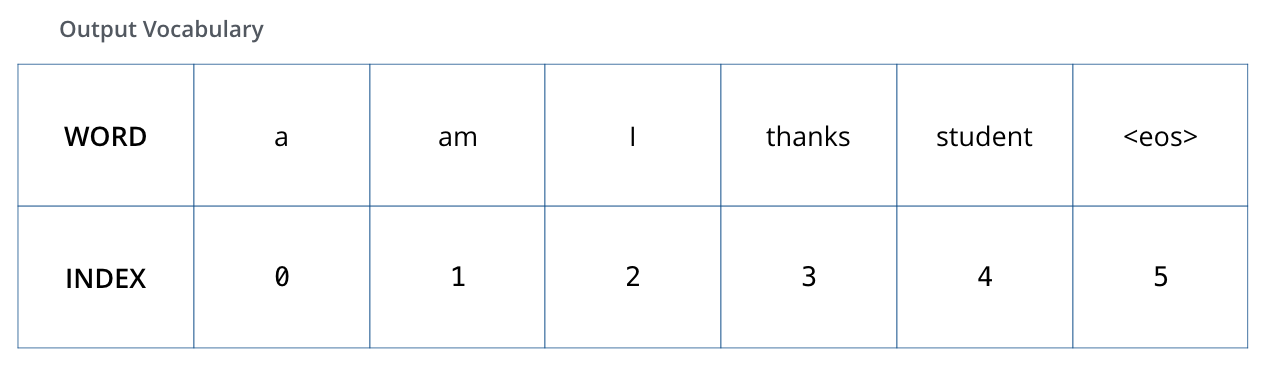
모델의 output vocabulary는 학습을 시작하기 전인 preprocessing 단계에서 완성됩니다. The output vocabulary of our model is created in the preprocessing phase before we even begin training.
이 output vocabulary를 정의한 후에는, 우리는 이 vocabulary의 크기만 한 벡터를 이용하여 각 단어를 표현할 수 있습니다. 이것은 one-hot encoding이라고도 불립니다. 그러므로 우리의 예제에서는, 단어 “am” 을 다음과 같은 벡터로 나타낼 수 있습니다: Once we define our output vocabulary, we can use a vector of the same width to indicate each word in our vocabulary. This also known as one-hot encoding. So for example, we can indicate the word “am” using the following vector:
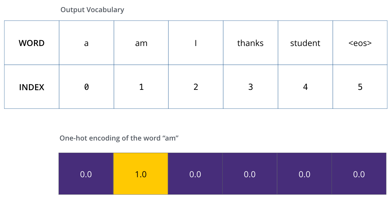
예제: 우리의 output vocabulary에 대한 one-hot encoding Example: one-hot encoding of our output vocabulary
이제 모델의 loss function에 대해서 얘기해보겠습니다 – 이것은 학습 과정에서 최적화함으로써 인해 모델을 정확하게 학습시킬 수 있게 해주는 값입니다. Following this recap, let’s discuss the model’s loss function – the metric we are optimizing during the training phase to lead up to a trained and hopefully amazingly accurate model.
Loss Function
The Loss Function
우리가 모델을 학습하는 상황에서 가장 첫 번째 단계라고 가정합시다. 그리고 우리는 학습을 위해 “merci”라는 불어를 “thanks”로 번역하는 간단한 예시를 생각하겠습니다. Say we are training our model. Say it’s our first step in the training phase, and we’re training it on a simple example – translating “merci” into “thanks”.
이 말은 즉, 우리가 원하는 모델의 출력은 “thanks”라는 단어를 가리키는 확률 벡터란 것입니다. 하지만 우리의 모델은 아직 학습이 되지 않았기 때문에, 아직 모델의 출력이 그렇게 나올 확률은 매우 작습니다. What this means, is that we want the output to be a probability distribution indicating the word “thanks”. But since this model is not yet trained, that’s unlikely to happen just yet.
학습이 시작될 때 모델의 parameter들 즉 weight들은 랜덤으로 값을 부여하기 때문에, 아직 학습이 되지 않은 모델은 그저 각 cell (word)에 대해서 임의의 값을 출력합니다. 이 출력된 임의의 값을 가지는 벡터와 데이터 내의 실제 출력값을 비교하여, 그 차이와 backpropagation 알고리즘을 이용해 현재 모델의 weight들을 조절해 원하는 출력값에 더 가까운 출력이 나오도록 만듭니다. Since the model’s parameters (weights) are all initialized randomly, the (untrained) model produces a probability distribution with arbitrary values for each cell/word. We can compare it with the actual output, then tweak all the model’s weights using backpropagation to make the output closer to the desired output.
그렇다면 두 확률 벡터를 어떻게 비교할 수 있을까요? 간단합니다. 하나의 벡터에서 다른 하나의 벡터를 빼버립니다. cross-entropy 와 Kullback–Leibler divergence를 보시면 이 과정에 대해 더 자세한 정보를 얻을 수 있습니다. How do you compare two probability distributions? We simply subtract one from the other. For more details, look at cross-entropy and Kullback–Leibler divergence.
하지만 여기서 하나 주의할 것은 우리가 고려하고 있는 예제가 지나치게 단순화된 경우란 것입니다. 조금 더 현실적인 예제에서는 한 단어보다는 긴 문장을 이용할 것입니다. 예를 들어 입력은 불어 문장 “je suis étudiant”이며 바라는 출력은 “i am a student”일 것입니다. 이 말은 즉, 우리가 우리의 모델이 출력할 확률 분포에 대해서 바라는 것은 다음과 같습니다: But note that this is an oversimplified example. More realistically, we’ll use a sentence longer than one word. For example – input: “je suis étudiant” and expected output: “i am a student”. What this really means, is that we want our model to successively output probability distributions where:
- 각 단어에 대한 확률 분포는 output vocabulary 크기를 가지는 벡터에 의해서 나타내집니다 (우리의 간단한 예제에서는 6이지만 실제 실험에서는 3,000 혹은 10,000과 같은 숫자일 것입니다).
- decoder가 첫 번째로 출력하는 확률 분포는 “i”라는 단어와 연관이 있는 cell에 가장 높은 확률을 줘야 합니다.
- 두 번째로 출력하는 확률 분포는 “am”라는 단어와 연관이 있는 cell에 가장 높은 확률을 줘야 합니다.
- 이와 동일하게 마지막 ‘
<end of sentence>‘를 나타내는 다섯 번째 출력까지 이 과정은 반복됩니다 (‘<eos>’ 또한 그에 해당하는 cell을 벡터에서 가집니다). *Each probability distribution is represented by a vector of width vocab_size (6 in our toy example, but more realistically a number like 3,000 or 10,000) *The first probability distribution has the highest probability at the cell associated with the word “i” *The second probability distribution has the highest probability at the cell associated with the word “am” *And so on, until the fifth output distribution indicates ‘<end of sentence>’ symbol, which also has a cell associated with it from the 10,000 element vocabulary.
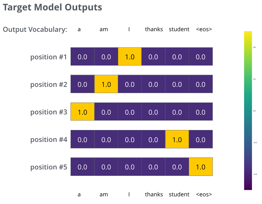
위의 그림은 학습에서 목표로 하는 확률 분포를 나타낸 것입니다. The targeted probability distributions we’ll train our model against in the training example for one sample sentence.
모델을 큰 사이즈의 데이터 셋에서 충분히 학습을 시키고 나면, 그 결과로 생성되는 확률 분포들은 다음과 같아질 것입니다: After training the model for enough time on a large enough dataset, we would hope the produced probability distributions would look like this:
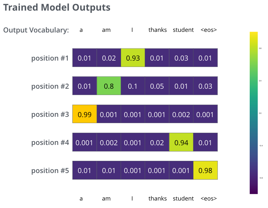
학습 과정 후에, 바라건대, 모델은 정확한 번역을 출력할 것입니다. 물론, 우리가 예제로 쓴 문장이 학습 데이터로 써졌다는 보장은 없습니다 (cross validation을 참고하세요). 그리고 한가지 여기서 특이한 점은, 학습의 목표로 하는 벡터들과는 달리, 모델의 출력값은 비록 다른 단어들이 최종 출력이 될 가능성이 거의 없다 해도 모든 단어가 0보다는 조금씩 더 큰 확률을 가진다는 점입니다 – 이것은 학습 과정을 도와주는 softmax layer의 매우 유용한 성질입니다. Hopefully upon training, the model would output the right translation we expect. Of course it’s no real indication if this phrase was part of the training dataset (see: cross validation). Notice that every position gets a little bit of probability even if it’s unlikely to be the output of that time step – that’s a very useful property of softmax which helps the training process.
모델은 한 타임 스텝 당 하나의 벡터를 출력하기 때문에 우리는 모델이 가장 높은 확률을 가지는 하나의 단어만 저장하고 나머지는 버린다고 생각하기 쉽습니다. 그러나 그것은 greedy decoding이라고 부르는 한가지 방법일 뿐이며 다른 방법들도 존재합니다. 예를 들어 가장 확률이 높은 두 개의 단어를 저장할 수 있습니다 (위의 예시에서는 ‘I’와 ‘student’). 그렇다면 우리는 모델을 두 번 돌리게 됩니다; 한 번은 첫 번째 출력이 ‘I’이라고 가정하고 다른 한 번은 ‘student’라고 가정하고 두 번째 출력을 생성해보는 것이죠. 이렇게 나온 결과에서 첫 번째와 두 번째 출력 단어를 동시에 고려했을 때 더 낮은 에러를 보이는 결과의 첫 번째 단어가 실제 출력으로 선택됩니다. 이 과정을 두 번째, 세 번째, 그리고 마지막 타임 스텝까지 반복해 나갑니다. 이렇게 출력을 결정하는 방법을 우리는 “beam search”라고 부르며, 고려하는 단어의 수를 beam size, 고려하는 미래 출력 개수를 top_beams라고 부릅니다. 우리의 예제에서는 두개의 단어를 저장 했으므로 beam size가 2이며, 첫 번째 출력을 위해 두 번째 스텝의 출력까지 고려했으므로 top_beams 또한 2인 beam search를 한 것입니다. 이 beam size 와 top_beams 는 모두 우리가 학습전에 미리 정하고 실험해볼 수 있는 hyperparameter들 입니다. Now, because the model produces the outputs one at a time, we can assume that the model is selecting the word with the highest probability from that probability distribution and throwing away the rest. That’s one way to do it (called greedy decoding). Another way to do it would be to hold on to, say, the top two words (say, ‘I’ and ‘a’ for example), then in the next step, run the model twice: once assuming the first output position was the word ‘I’, and another time assuming the first output position was the word ‘me’, and whichever version produced less error considering both positions #1 and #2 is kept. We repeat this for positions #2 and #3…etc. This method is called “beam search”, where in our example, beam_size was two (because we compared the results after calculating the beams for positions #1 and #2), and top_beams is also two (since we kept two words). These are both hyperparameters that you can experiment with.
더 깊이 Transformer 알아보기
Go Forth And Transform
이 글이 Transformer의 주요 개념들을 대략적으로 잘 설명한 소개 글이 되었길 바랍니다. 만약 Transformer에 대해 더 자세히 알고 싶으시다면 다음 자료들을 추천합니다: I hope you’ve found this a useful place to start to break the ice with the major concepts of the Transformer. If you want to go deeper, I’d suggest these next steps:
- Attention Is All You Need 논문과 구글에서 작성한 공식 Transformer 블로그 글 (Transformer: A Novel Neural Network Architecture for Language Understanding)을 읽으세요. Tensor2Tensor 발표 글 도 추천합니다.
- 모델과 세부사항들을 설명하는 저자 Łukasz Kaiser의 발표를 시청하세요.
- Tensor2Tensor repository의 부분으로서 제공된 Jupyter Notebook을 가지고 놀아보세요.
- Tensor2Tensor repo를 둘러보세요.
*Read the Attention Is All You Need paper, the Transformer blog post (Transformer: A Novel Neural Network Architecture for Language Understanding), and the Tensor2Tensor announcement. *Watch Łukasz Kaiser’s talk walking through the model and its details *Play with the Jupyter Notebook provided as part of the Tensor2Tensor repo *Explore the Tensor2Tensor repo.
Transformer를 활용한 follow-up 연구들로는 다음이 있습니다: Follow-up works:
- Depthwise Separable Convolutions for Neural Machine Translation
- One Model To Learn Them All
- Discrete Autoencoders for Sequence Models
- Generating Wikipedia by Summarizing Long Sequences
- Image Transformer
- Training Tips for the Transformer Model
- Self-Attention with Relative Position Representations
- Fast Decoding in Sequence Models using Discrete Latent Variables
- Adafactor: Adaptive Learning Rates with Sublinear Memory Cost
감사의 말
Acknowledgements
이 글의 초기 버전에 피드백을 주신 Illia Polosukhin, Jakob Uszkoreit, Llion Jones , Lukasz Kaiser, Niki Parmar, and Noam Shazeer에게 감사를 전합니다. Thanks to Illia Polosukhin, Jakob Uszkoreit, Llion Jones , Lukasz Kaiser, Niki Parmar, and Noam Shazeer for providing feedback on earlier versions of this post.